- New high precision reference oscillator
- High current transformer driver
- Improved low temperature dependence drive
transformer
- Magnetic modulator input for measuring frequency
response
- Electrostatic modulator input for measuring
frequency response
- GGP low pass filter
- Improved layout with 4 layer PCB and shielded
input stage
- On-board temperature sensors
- Improved components
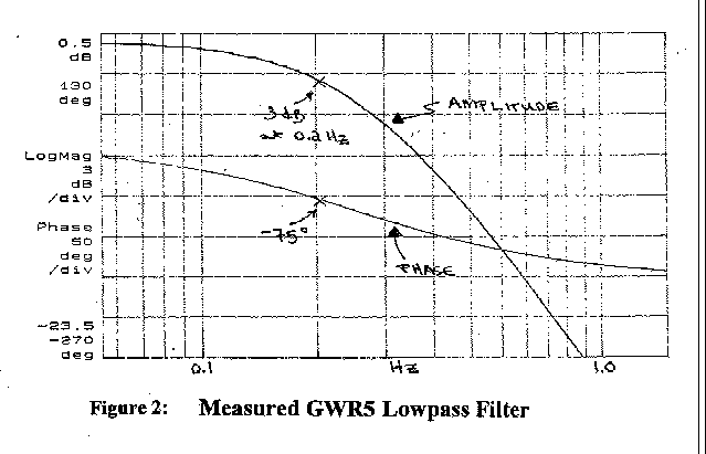
- GWR5 Low Pass Filter
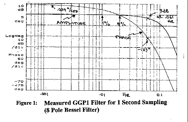
- GGP1 filter intended for 1 Hz sampling rate -
(See Figure 1)
- 8 pole Bessel filter
- Corner frequency at 61.5 mHz (16.3 sec
period)
- Constant time delay of 8.2 seconds (Phase
lag 0.034 deg/cpd)
- 100 dB attenuation at 0.5 Hz (fnyq
for 1 Hz sampling)
- Attenuation < 1% (-.086dB) below 0.01
Hz (100 sec period)
- Attenuation < 4% (-.341dB) below 0.02
Hz (50 sec period).
- GGP2 filter intended for 0.5 Hz sampling rate
(optional)
- 8 pole Bessel filter
- Corner frequency at 30.8 mHz (32.6 sec
period)
- Constant time delay of 16.4 seconds
(Phase lag 0.068 deg/cpd)
- 100 dB attenuation at 0.25 Hz (fnyq
for 0.5 Hz sampling)
- Attenuation < 1% (-.086dB) below 0.005
Hz (200 sec period)
- Attenuation < 4% (-.341dB) below 0.01
Hz (100 sec period).
- Magnetic modulator
- Adder allows injection of current into
the feedback circuit, to measure closed
loop response.
- Jumper selection removes adder
eliminating unnecessary components.
- Jumper selection allows both open and
closed loop characterization.
- Electrostatic modulator
- Allows similar measurements by using
electrostatic force
- Response depends only on geometry of
sphere & plates and is independent of
magnetic levitation.
- Allows measurement of charge.
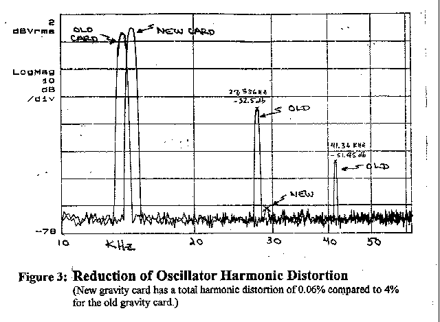
- Improved oscillator - (See Figure 3)
- Improved temperature stability
- Reduced harmonic distortion
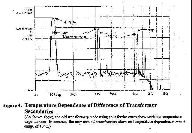
- Improved drive transformer - (See Figure 4)
- Toroid design replaces bobbin design
decreasing TC by order of magnitude.
- High current transformer driver
- Lowers distortion and impedance of drive
circuit
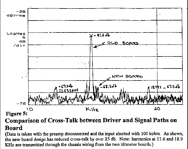
- 4 layer PCB, improved grounding and shielded
input stage
- Reduced cross-talk between drive and
sense circuits - (See Figure 5)
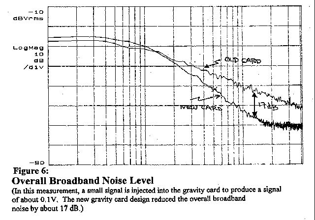
- Reduced overall broad band noise - (See Figure 6)
- On-board temperature sensors
- Simplifies monitoring of electronics
temperature
- Improved components
- Hermetically sealed ultra stable passive
components
- Selected grade IC's for low noise,
thermal drift, and long term stability
- Conformal coating improves resistance to
humidity and surface contamination
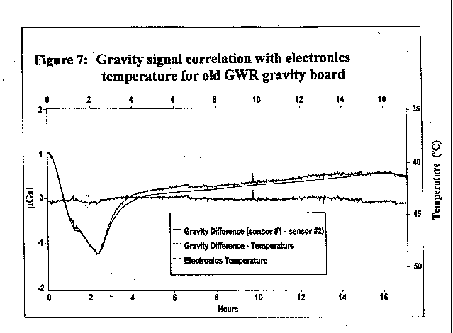
- Old gravity card had a
temperature dependence between 0.1 to 1 mgal/°C. (See Figure
7)
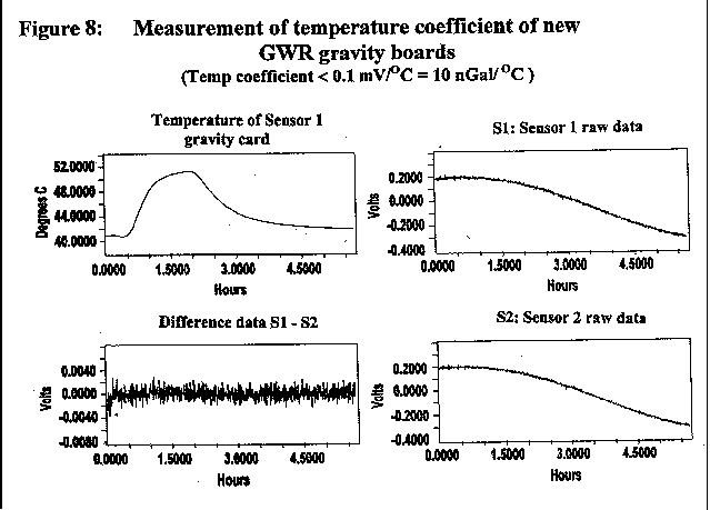
- New gravity cards have
temperature dependence less than 0.01 mgal /
°C (See Figure 8)
- Intended for future acquisition system capable of
sampling at approximately 1 plc (50Hz or 60Hz).
Data system should implement real-time digital
filter decimating output to 1 Hz.
- 2 pole Bessel filter
- Corner frequency at 200 mHz (5 sec. period).
- Check feedback
characteristics
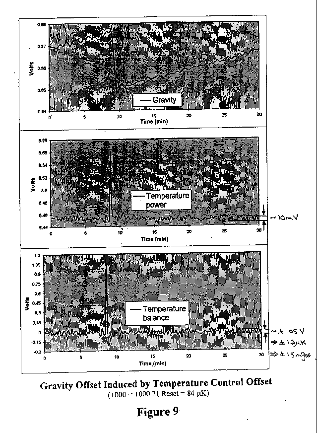
Uses should measure the response of gravity,
temperature power and temperature balance to a
change in temperature control null position. In Figure
9, an offset from
``off" to +000 (=0.21 reset) equals about
.084 mK and produces a gravity offset of 1.25
mgal.
When the feedback is working well, both the
temperature power and balance should return to
equilibrium with only 1 to 2 excursions.
- Expected temperature
balance noise (and what gravity noise level this
corresponds to)
Temperature balance noise is about ± 0.05
mV
=> ± 1.5 mK => 15 ngal
- What are the implications
of spikes on heater power or temperature balance
signals? Could these produce offsets in data?
Spikes in the temperature power or balance could
indicate that an offset in temperature has
produced an offset in gravity. In concept, one
could measure an offset in power associated with
the temperature offset. However, noise limits
measurement of power offsets to 10 mV. Therefore,
since the power sensitivity is only 0.4 mV/mgal, one
can only resolve offsets larger than 25 mgal.
- Can the spikes be recorded
to indicate a problem?
Yes, one must correlate gravity offsets to power
spikes to prove cause and effect. However, this
requires at least a 2 second sampling interval
since the power spikes are only 10-15 seconds
wide.
- Check feedback
characteristics
Users should measure the response of tile power
and tilt balance to a change in both X and Y
reset. In Figure 10 the X Reset has been changed from
+521 to +526 which corresponds to about 30 mradian.
Check that both the power and balance return to
equilibrium with only 1 or 2 oscillations.
- Expected tilt balance noise
The tilt noise will depend on how quiet the
user's site is. At GWR the tilt balance noise is
about ± 10 mV which corresponds to a tilt noise
of about ± 0.1 mradian. Users are encourage to
measure the relationship between micrometer
``mils", tilt balance volts (BD=7), reset
units and mradian. In the instrument tested at
GWR: 1 mil = 2.9 V = 5.8 reset = 32 mradian.
These relationships will depend on the length of
the tilt arms, the electronic gain, and the
tiltmeter sensitivity.
- What are the implications
of spikes on X or Y tilt power or balance
signals? Could these produce offsets in data?
As with temperature, these spikes could indicate
that changes in the tilt control position are
producing offsets. However, such a conclusion
cannot be reached without using secondary
tiltmeters or by correlation of spikes with
gravity offsets. The width of tilt balance spikes
is 2 to 4 minutes and can easily be observed by
sampling with a 20 second interval.
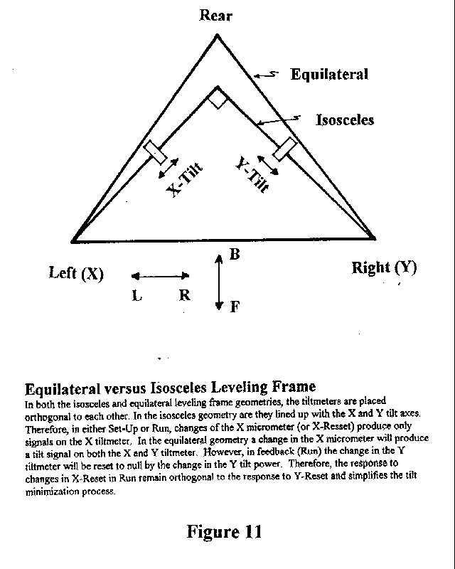
- Tilt geometry & manual
tilt desensitizing (FB & LR)
All compact Dewars and many other instruments now
use equilateral leveling frames versus the older
isosceles triangular frames. The geometry of the
two systems is illustrated in Figure
11. The advantage
of the isosceles support frames is that the left
and right axes are orthogonal and that the two
tiltmeters can be aligned with these axes. In
SET-UP, this means that reading of the X (or Y)
micrometer does not affect the null position
measured with the other micrometer. With the
equilateral frame, the user must simultaneously
use both left and right micrometers to define two
new tilt axes labeled Left-Right (LR) and
Forward-Back (FB). LR is defined by moving both X
and Y micrometers in the same direction, e.g.:
DELTA X = +5 mils and DELTA Y = +5 mils; while FB
is defined by moving in opposite directions,
e.g.: DX = +5 mils and DY = -5
mils.
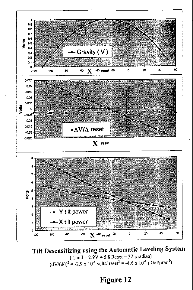
- Tilt desensitizing in
feedback using X or Y Resets
With the leveling platform operating in feedback
(RUN), both equilateral and isosceles support
frames can be tilt minimized in an orthogonal
fashion using the Left (X) Reset and the Right
(Y) Reset. The X & Y reset functions produce
orthogonal tilts because they produce electronic
offsets in the tiltmeters themselves. However,
since the thermal levelers do not produce
orthogonal tilts, they both must respond to
either a X or Y Reset change. This is shown in Figure
12, where the X
tilt axis is being tilt minimized using only the
X-Reset. As shown, the X Power response is larger
than the Y power. From the geometry of the
equilateral frame and tiltmeter alignment, the
ratio of the Y tilt power should be 0.27. In the
example, the power ratio was 0.36 which is most
likely due to errors in the electronic square
root function in the feedback network and to
different leveler response to heat.
Expected
tilt noise close to minimum
The slope of the tilt curve Dg/( D Reset)2
can be used to calculate the expected gravity
noise produced by tilts. For example, in the data
show, the gravity noise is about:
DgN @ 4.6 x 10⁻⁴ (mgal/(mrad)2)(Q-Q0) DQ (1)
Therefore, the
tilt noise depends on the tilt slope, how close the
instrument is adjusted to the tilt null Q0 and
the noise level DQ at the site. In the example shown, if (Q-Q0 <
1 Reset (=5mrad) and the noise DQ = 0.1mrad,
then the tilt induced gravity noise DgN @ 2.5 ngal.
At a site such as Membach, the tilt noise is about 5
times quieter than at GWR. Therefore, the tilt
induced gravity noise will be DgN
(Membach) @ 0.5 ngal
- Need for an annual tilt
check
GWR recommends that users perform annually tilt
checks for both X-Reset and Y-Reset. When the
system is operating properly, neither the X or Y
Reset values will change in time. This means that
the tilt minimum of the gravity meter and the
null points of the tiltmeters have remained
stationary with time.
- (Membach,
Belgium data as an example)
- Instrumental channels to record gravity and
for SG maintenance
Data channels can be classified into three
categories. Recording the main signals of gravity
and air pressure is already fully discussed in
previous GGP meetings. The auxiliary signals are
used to check and monitor the subsystems of the
gravimeter to make sure they are operating
correctly. It is important to establish a
baseline of operation on the subsystems for
regular comparison to make sure performance does
not degrade in time. This will be especially
helpful when problems arise that must be
discussed with GWR. Comparison of data with the
system working correctly versus improper
operating is essential for diagnosing failures
rapidly. The geophysical signals are of prime
importance for correlating with observed gravity
changes. This correlation allows further
reduction of secular or short term signals from
the data. For example, groundwater will produce
long term secular signals; while rain fall may
produce 1 to 3 day spikes in the data. Finally,
regular absolute gravity measurements allow
either confirmation of long term trends in
superconducting data or correction of
instrumental drift.
- Main signals:
Gravity
Air pressure
- Temperature balance
Heater power
X & Y Tilt balance
X & Y Tilt power
Electronics temperature
Vault temperature
Neck temperatures
Helium flow
(Compressor water coolant temperatures)
(mode data?)
- Geophysical signals:
Permanent GGP measurement of elevation changes
Ground water variations
Soil moisture
Rain and snowfall
Other??
- Periodic Absolute Gravity measurements
- Notes of caution:
1) User's data systems should use
differential and isolated inputs. Each
signal from the GEP-2 electronics has a
corresponding return (common) which is referenced
to a specific location on the board where the
signal is generated. Connecting commons together
at the data system will disrupt the electronic
design and will produce ground currents and
noise. It is for this reason that GJ1 through GJ4
and the front panel connector are isolated BNC
connectors. The commons of these BNCs should not
be grounded.
2) Use caution on recording Heater Power.
We have observed that connecting a long cable to
the heater power (GJ5 pins 7/15) can cause noise
on the gravity signal. Pin 7 connects directly to
the output of the temperature feedback integrator
(U7). The increased capacitance to ground present
in the cable connected to pin 7 may cause U7 to
oscillate at a high frequency. This oscillation
will shift the DC level of the output and produce
a shift in the temperature control position. If
this happens rapidly the result looks like noise.
If it happens infrequently it will look like
random offsets on the gravity meter. Users with
short leads between GEP-2 and their data systems
are probably safe from oscillations. However, for
users with long leads we recommend that they
discontinue recording the heater power by
disconnecting pins 7/15 in the cable connected to
GJ5.
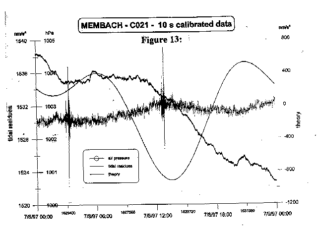
- Daily & weekly analysis of data
Daily - It is important to analyze and
monitor the main and auxiliary signals frequently
in order to minimize data interruptions and gaps.
The best way to guarantee the highest quality
gravity data is to generate a tidal residual
signal by subtracting a tide model based on the
analysis of previous data. Ideally this can be
done on a daily basis as in the data shown in Figure 13 (air
pressure, tidal residual, & theory from
Membach). Once the residual is generated, the
user can determine:
1) Has the instrumental noise level remained low?
2) Are there any offsets or spikes (besides
earthquakes)?
3) Are there any abrupt changes in slope or
drift?
4) Is the data system, timing and data storage
working properly?
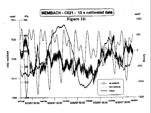
Weekly - The same type of analysis can
be done on a weekly basis as in the data shown in
Figure 14 (air
pressure, tidal residual & theory from
Membach). This residual data should be compared
to the X & Y Tilt balance and power (Figure 15), Heater
power and temperature balance (Figure 16),
electronics temperature, and vault temperature.
For example on the X tilt power there is a large
spike. However, by comparison of this event to
the tidal residual one can determine that this
event did not produce a corresponding spike or
noise on the residual data. What caused this
spike then? If it was a user entering the vault,
it should cause a change in vault temperature or
produce an entry into the log book.
Clearly, the more often the tidal residual is
generated and checked the shorter gaps in the
data will be. However, weekly checks of the
temperature, tiltmeters, and refrigeration
systems are most likely adequate. Monitoring the
neck thermometers to observe an increase in
temperature is the most rapid way to determine
when the cold head is beginning to age. This
allows plenty of time to replace the cold head
since they degrade slowly.
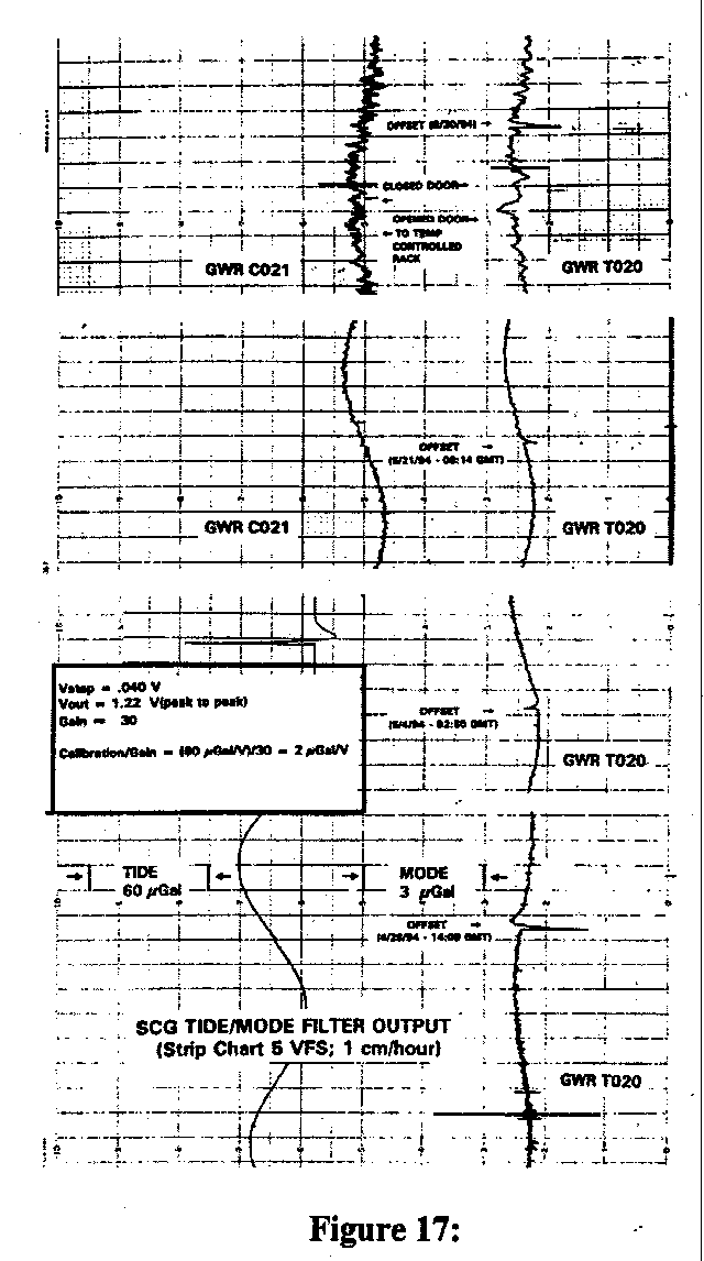
- Is the Mode filter useful anymore?
Recording the mode bandpass filter on a strip
chart recorder (See Figure
17) is a quick and simple way to examine the
high frequency noise present on the gravity
signal. Therefore, it may be useful for users who
are not generating and examining daily tide
residuals. However, it can only be used for
checking for changes in instrumental noise and
for offsets and spikes. It cannot be used for
changes in drift (since DC signals are filtered
out) or for operation of the data system or
storage medium.
The mode filter could be recorded as auxiliary
data at 20 second intervals and be used to scan
the data for offsets. As shown in Figure 17, a 40 mV
step function into the mode filter produces a
spike response of about 1.22 V (peak to peak).
Therefore, the magnitude of offsets producing
such spikes can be (practically) read of the mode
filter data if the noise level is low. For high
noise regions it is more difficult to remove such
offsets. Possibly, the mode filter data would be
useful to other GGP participants to quickly
determine data quality before they commit to the
process of ``cleaning" the data for further
analysis.
- Importance of Absolute Gravity Measurements
Figure 18 shows
the gravity residuals of the superconducting
gravimeter (SG) compared to the measurements from
the absolute gravimeter (AG) at Membach, Belgium.
In this case there was a data gap and offset that
occurred in the SG near the end of May-96. This
offset was estimated and corrected by comparison
of SG to AG data. From these data sets it appears
that the SG at Membach has very little
instrumental drift. Generally, however, some
drift may be present on the SG at other sites.
Such drifts are always monotonic and usually
decrease in time. These drifts can be measured by
comparison of the SG residual data to AG data if
AG is taken at regular periodic intervals. The SG
can also be used to check proper operation of the
AG. As can be seen from the data, there are two
AG data points at 18000 hours that disagree
significantly with the rest of the data.
- Importance of measuring other geophysical data
The agreement of SG and AG data markedly
increases confidence in both data sets and proves
that the observed gravity variations are of
geophysical origin and not of instrumental
origin. The geophysicist's job is now to identify
the cause of such variations. One common method
of doing this is by establishing a correlation
between the gravity residual and other
geophysical signals. However, this powerful
technique can only be used if the geophysical
signals have been recorded over the same time
period as the gravity data itself! Therefore,
users must establish a list of geophysical
signals that are most likely to influence data at
their sites and implement methods to measure and
record them as soon as possible.
Acknowledgment: The author sincerely thanks
Olivier Francis and Marc Hendrickx for supplying
the data from Membach, Station, Belgium which is
used as examples in this section.
- GOP recommends accuracy better than 0.1 hPa.
- Admittance of air pressure to gravity is about 3
nms2 / hPa.
- GOP recommends measuring to accuracy of
0.3nms2
- Best transducers are stable to no better than 0.1
bPa / year.
- To maintain GOP specification, calibration on
yearly basis is required.
- Calibration by factory with dead weight
tester.
- Calibration in the field with transfer
meter.
Quartz Bourdon Tube
- Mainly for Laboratory standard
- Very Expensive.
- Vibrating Cylindrical oscillator (Weston or
Schlumberger. sensor)
- Long history of stable measurements
- Sensitive to changes in media density
(humidity).
- Silicone Resonant Pressure Transducer (e.g. RPT
by Druck)
- Newest Technology
- Stable, accurate, insensitive to media
- Capacitance bridge (e.g. MKS Baratron)
- Best suited for low pressure (vacuum)
- Vibrating Cylindrical Oscillator and RPT sensors
are intrinsically digital
- Changes in Pressure effect the frequency
of a resonating structure
- Conversion to an analog signal is an
unnecessary step and degrades the system
stability
- Data should be collected digitally which
may require modification of data
acquisition software.
Comparison of various types of
pressure transducers
| |
Temp.
Controlled Capacitive Sensor (MKS Baratron) |
Silicone
Resonant Pressure Transducer (RPT Druck) |
Vibrating
Cylinder (Weston or Schiumberger sensor) |
| Accuracy |
1.5 hPa |
0.1 hPa |
0.1 hPa |
| Drift |
not
specified |
0.1 hPa /
year |
0.1 hPa /
year |
| Operating
temp. range |
+15°C
/ +40°C |
-20°C
/ +60°C |
-40°C
/ +70°C |
| Temperature induced
errors |
0.3 hPa / °C |
0.2 hPa over full
temperature range |
better than stated
accuracy |
| Humidity sensitive |
NO |
NO |
YES |
| output format |
analog (DCV) |
digital (R5232/R5422
selectable) |
digital (R5232 OR
R5422) |
| DC! Gain calibration |
Evacuate! dead weight
test |
dead weight test |
dead weight test |
| Typical usage |
low pressure |
general barometric |
barometric |
| History |
|
Recently developed |
Long History, industry
standard |
- All GGP participants should upgrade pressure
transducers to either the RPT or Vibrating
Cylinder type
- Data should be collected digitally via a serial
port rather than through an analog channel
- GWR now recommends a Silicone Resonant Pressure
Transducer manufactured by Druck Instruments
- GWR (or other?) could maintain a calibrated
transfer meter for use by GGP participants if the
community desires it
- Refrigeration system is the most maintenance
intensive part of the SG system!
- Compressor adsorber replacement every 10,000
hours (13 months)
- Annual coldhead clearance check
- Coldhead maintenance approximately every 20,000
hours
- Compressor cooling must be maintained within
specified limits
- Evaluate heat management criteria
carefUlly when setting up the system
- Choose proper cooling system for ambient
conditions
- Monitor cooling water temperatures
- Failure to provide adequate cooling will
eventually result in premature compressor failure
- In some cases inadequate cooling can result in
oil contamination to the entire cooling system
including the gas hoses and coldhead!
- APD HC2 Compressor specifies cooling water is
maintained within certain limits!
- 2.3 liters / minute minimum flow rate
- 27 "C maximum inlet temperature
- Approximately 1.8 kW of heat rejection is
required.
- Dry type coolers
- Operate by passing water to be cooled
through tubes attached to cooling fins.
Fans force ambient air over fins to
remove heat
- These coolers will never cool to
the ambient air temperature, cooling to
within 5 "C to 10 "C of ambient
is typical
- Inexpensive, simple, reliable
- Compressor driven chillers
- Operate with freon or other compressed
gas (like a home refrigerator or air
conditioner)
- Require additional electrical power
- Can maintain cooling water at temperature
far below ambient air temperature
- APD Cool-Pack 4
- Dry type cooler
- Maintains cooling water inlet to HC2
approximately 5°C
above ambient
- Acceptable when ambient air temperature
does not exceed 22"C
- GWR AW75 Cooler
- Dry type cooler
- Maintains cooling water inlet to HC2
approximately 4 °C
above ambient
- Acceptable when ambient air temperature
does not exceed 23°C
- Increased pump capacity decreases
compressor outlet temperature maintaining
increased safety margin
- Heavy duty pump, fan, and heat exchanger
for increased reliability
- Schreiber 1 Ton Compressor Driven Water
Chiller
- Compressed freon refrigerator maintains
low temperatures in extreme ambient
conditions (up to 45°C)
- Rated for outdoor use
- Low ambient controls allows operation in
sub zero conditions
- Large water reservoir reduces
refrigeration cycling improving
reliability
RECOMMENDATION -
Purchase suitable water chiller from your local
refrigeration expert!
|