Location

2020/10/30 11:51:27 37.92 26.79 21

Moment Tensor Comparison

The following compares this source inversion to the USGS Rapid Moment Tensor Solution and to the Harvard CMT solutions, if they are available.

SLU	SLU RMT	USGS	USGS
Moment Tensor Solution ENS 2020/10/30 11:51:27:0 37.92 26.79 5.0 7.0 Greece Best Fitting Double Couple Mo = 3.35e+26 dyne-cm Mw = 6.95 Z = 5 km Plane Strike Dip Rake NP1 78 73 -100 NP2 290 20 -60 Principal Axes: Axis Value Plunge Azimuth T 3.35e+26 27 177 N 0.00e+00 10 82 P -3.35e+26 61 333 Moment Tensor: (dyne-cm) Component Value Mxx 2.01e+26 Mxy 1.60e+25 Mxz -2.63e+26 Myy -1.50e+25 Myz 7.19e+25 Mzz -1.86e+26 ############## ###################### #####---------------######## ##-----------------------##### ##---------------------------##### #-------------------------------#### -------------- ------------------### --------------- P -------------------### --------------- --------------------## ------------------------------------------ -------------------------------------###-- ---------------------------------########- ----------------------------#############- #------------------##################### ######################################## ###################################### #################################### ################################## ############## ############# ############# T ############ ########## ######### ############## Global CMT Convention Moment Tensor: R T P -1.86e+26 -2.63e+26 -7.19e+25 -2.63e+26 2.01e+26 -1.60e+25 -7.19e+25 -1.60e+25 -1.50e+25	SLU RMT SLU USGS/SLU Moment Tensor Solution ENS 2020/10/30 11:51:27:0 37.92 26.79 21.0 7.0 Greece Stations used: GE.CSS HL.ATH HL.EVR HL.GVD HL.IACM HL.ITM HL.KARP HL.KLV HL.KSL HL.KTHA HL.KZN HL.NEO HL.NVR HL.SIVA HL.SKY HL.SMTH HL.TETR HL.VAM HL.VLY HT.AGG HT.ALN HT.AOS2 HT.EVGI HT.GRG HT.KAVA HT.KNT HT.KPRO HT.NEST HT.OUR HT.PAIG HT.RTZL HT.SOH HT.SRS HT.THAS HT.THE HT.TYRN HT.XOR KO.AFSR KO.ARMT KO.BALB KO.BGKT KO.CTYL KO.EDC KO.GEML KO.HDMB KO.ISK KO.KAMT KO.KAVV KO.KCTX KO.KIZT KO.KONT KO.KULU KO.KURC KO.LADK KO.LFK KO.LOD KO.RKY KO.RUZG KO.SAUV KO.SDAG KO.SHUT KO.SILT KO.SVRH KO.YALI KO.YLV MN.ISP MN.KEK MN.THL Filtering commands used: cut o DIST/3.3 -80 o DIST/3.3 +150 rtr taper w 0.1 hp c 0.01 n 3 lp c 0.02 n 3 Best Fitting Double Couple Mo = 2.37e+26 dyne-cm Mw = 6.85 Z = 8 km Plane Strike Dip Rake NP1 268 45 -95 NP2 95 45 -85 Principal Axes: Axis Value Plunge Azimuth T 2.37e+26 0 1 N 0.00e+00 4 271 P -2.37e+26 86 93 Moment Tensor: (dyne-cm) Component Value Mxx 2.37e+26 Mxy 6.12e+24 Mxz 1.27e+24 Myy -7.43e+23 Myz -1.46e+25 Mzz -2.36e+26 ###### T ##### ########## ######### ############################ ############################## ################################## ###########---------------########## #######-------------------------###### #####-------------------------------#### ###-----------------------------------## ##--------------------------------------## ----------------------- ---------------- ##--------------------- P ---------------- ###-------------------- ---------------# ####-----------------------------------# ######------------------------------#### ########-------------------------##### ############---------------######### ################################## ############################## ############################ ###################### ############## Global CMT Convention Moment Tensor: R T P -2.36e+26 1.27e+24 1.46e+25 1.27e+24 2.37e+26 -6.12e+24 1.46e+25 -6.12e+24 -7.43e+23 Details of the solution is found at http://www.eas.slu.edu/eqc/eqc_mt/MECH.NA/20201030115127/index.html	Body-wave Moment Tensor (Mwb) Moment 2.546e+19 N-m Magnitude 6.87 Mwb Depth 8.0 km Percent DC 80% Half Duration - Catalog US Data Source US 4 Contributor US 4 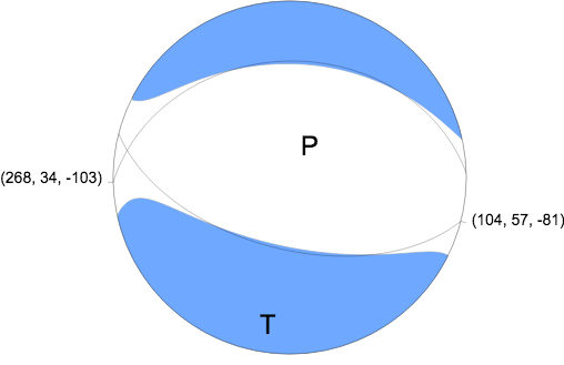Nodal Planes Plane Strike Dip Rake NP1 268 34 -103 NP2 104 57 -81 Principal Axes Axis Value Plunge Azimuth T 2.670e+19 N-m 11 188 N -0.269e+19 N-m 7 279 P -2.401e+19 N-m 76 42	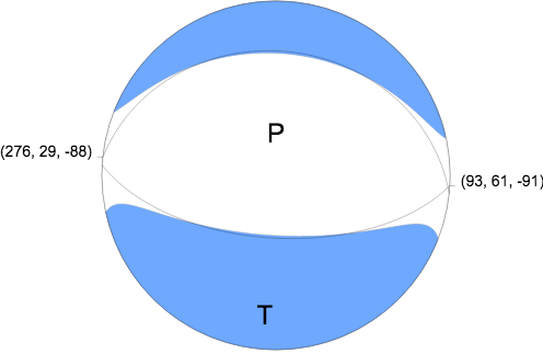W-phase Moment Tensor (Mww) Moment 4.087e+19 N-m Magnitude 7.01 Mww Depth 11.5 km Percent DC 85% Half Duration 8.39 s Catalog US Data Source US 4 Contributor US 4 Nodal Planes Plane Strike Dip Rake NP1 93 61 -91 NP2 276 29 -88 Principal Axes Axis Value Plunge Azimuth T 4.241e+19 N-m 16 184 N -0.328e+19 N-m 1 94 P -3.913e+19 N-m 74 0

USGS finite fault inversion

The USGS final fault solution is given at https://earthquake.usgs.gov/earthquakes/eventpage/us7000c7y0/finite-fault?source=us&code=us7000c7y0_1. This solution pefers the EW striking nodal plane but assumes a source depth of 21 km.

Data set

The following broadband stations passed the QC and were used for the source inversion. AAK ABPO ALE ASCN BBSR BILL BORG BORK CHTO CMLA COLA DGAR EDA FDFM FFC FOMA FURI HRV INCN IVI KBL KEV KURK LVZ MA2 MACI MAKZ MBAR MPG MSEY NIL PALK PET RCBR RER ROCAM SACV SFJD SHEL SOK SSPA SUR TATO TIXI TLY TSUM ULN WUS YAK YSS

Grid Search

All observed and Greens function waveforms are corrected to instrument response to ground velocity in meters/sec for the passband of 0.004 - 5 Hz. The traces were then lowpass filtered at 0.25 Hz and interpolated to a sample rate of 1 second.

For the grid search, the observed traces and Green's functions are read in an cut using the following commands

Processing parameters

#####
#	Driver script for the teleseismic waveform inversion
#
#	The depth HS must be of the form 0010 for a depth of 1.0 km
#       of 6700 for a depth of 670.0 km
#
#	The Filter_Band is an integer with the following meansing
#
#	FILTER_BAND	1/FH	1/FL
#	1		60	12	for Mw < 6.4
#	2		100	20	6.4 =< Mw < 6.8 
#	3		120	40	6.8 =< Mw < 7.2 
#	4		143	80	7.2 =< Mw < 9.3 
#####
#	Source duration - halfwidth of triangular function
#	this filters only the Green functions
#
#	halfwidth = 1.05 * 10-8 * M0^1/3 (M0 is dyne-cm)
#
#	MW	   half-width (sec)
#	5.0         0.75
#	6.0         2.45
#	7.0         7.7
#	8.0        24.5
#	9.0        74.3
#                       0.5*(MW - 9)
#  or half-width=74.3*10
#  or echo 6.93 |  awk '{print 74.3*exp(0.5*log(10.0)*(0050 - 9.0)) }'
#####
#  Processing window for P (use SAC variable A for P arrival
#  	Start   A  - 30
#  	End     A  + 2*HALFWIDTH + 0.03*HS + 30 + 1/FH +100
#  Processing window for SH (use SAC variable T0 for SH arrival
#  	Start   T0 - 60
#  	End     T0 + 2*HALFWIDTH + 0.06*HS + 30 + 1/FH +170
#  Processing window for SV (use SAC variable T1 for SV arrival
#  	Start   T1 - 60
#  	End     T1 + 2*HALFWIDTH + 0.06*HS + 30 + 1/FH +170
#	
#	The term involving HS serves to include the depth phases and
#	to exclude the PP or SS at most distanace
#####

The waveforms are then bandpass filtered by the application of the following high- and low-pass stages (an optional microseism filter):

hp c 0.0083 2
lp c 0.0250 2
int
br c 0.12 0.25 n 4 p 2

The source inversion is a multipass operation since a lower frequency filter band is used for larger earthquakes and since a search is made over depth. Up to three passed of the outer loop are made, after which the moment magnitude is determined and filter settings readjusted. The inner loop over depth samples all depths from 0 to 800 km with 5 km increments in depth to 50 km, followed by 10 km depth sampling for the remaining range.

The following filter ranges are used according to the moment magnitude Mw:

   FILTER_BAND   1/FH(s)  1/FL(s)
       1           60     12      Mw < 6.4
       2          100     20      6.4 < Mw <= 6.9
       3          120     40      Mw > 6.9

The map displays the distribution of stations used for this source inversion.

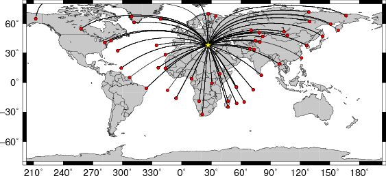
Location of the earthquake (yellow star) and great circle path from the epicenter to each station (red) [created using GMT (Wessel, P., and W. H. F. Smith, New version of Generic Mapping Tools released, EOS Trans. AGU, 76 329, 1995.)]

For this data set the favored solution is

WVFGRD96    5.0   290    20   -60   6.95 0.5032

The following figures show the sensitivity of the goodness of fit parameter so source depth, the waveform comparison as a function of epicentral distance in degrees and the source to station azimuth

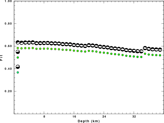
Depth Sensitivity

Goodness of fit as a function of source depth. The measure is 1 - SUM (o -p)2 / SUM o2. A value of 1.0 is the best fit. The best double couple mechanism for the solution depth is plotted above goodness of fit value to indicate how the mefhanism may change with depth.

Detailed Waveform Comparison

P-wave Z component

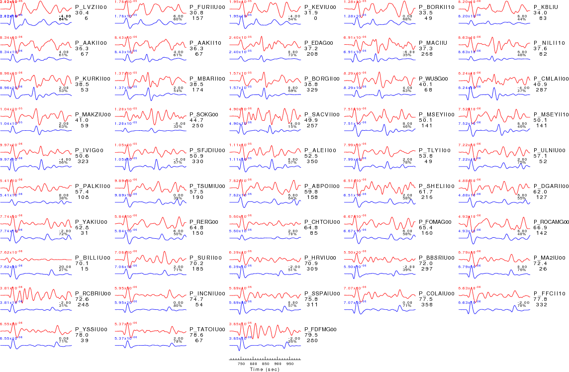
Comparison of the observed traces (red) and solution predicted traces (blue) ordered in terms of increasing epicentral distance. Each pair of traces is annotated with the station name, epicentral distance in degrees, source to station azimuth in degrees. Each pair of traces is plotted with the same scale and the peak amplitudes are indicated at the lect of each trace. Finally the time shift between the P-wave first arrival picked and the the theoretical P-wave first arrival in the predicted trace is indicated, with a positive sign indicating that the predicted trace has been shifted to the right by the given number of seconds. as a function of source to station azimuth in degrees (D). The purpose of this display is to highlight the azimuthal dependence on the first motion. The traces are annotated with the station name at the top.

SH-wave T component

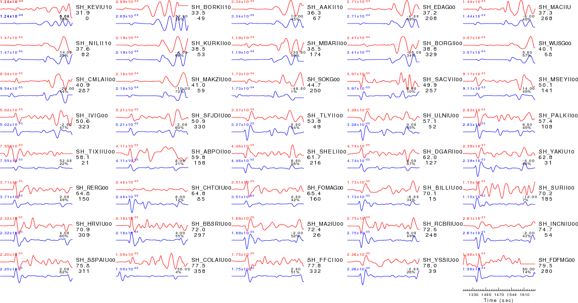
Comparison of the observed traces (red) and solution predicted traces (blue) ordered in terms of increasing epicentral distance. Each pair of traces is annotated with the station name, epicentral distance in degrees, source to station azimuth in degrees. Each pair of traces is plotted with the same scale and the peak amplitudes are indicated at the lect of each trace. Finally the time shift between the P-wave first arrival picked and the the theoretical P-wave first arrival in the predicted trace is indicated, with a positive sign indicating that the predicted trace has been shifted to the right by the given number of seconds. as a function of source to station azimuth in degrees (D). The purpose of this display is to highlight the azimuthal dependence on the first motion. The traces are annotated with the station name at the top.

SV-wave R component

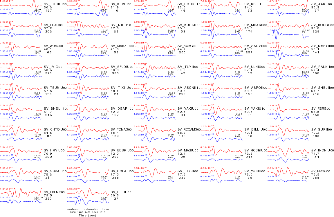
Comparison of the observed traces (red) and solution predicted traces (blue) ordered in terms of increasing epicentral distance. Each pair of traces is annotated with the station name, epicentral distance in degrees, source to station azimuth in degrees. Each pair of traces is plotted with the same scale and the peak amplitudes are indicated at the lect of each trace. Finally the time shift between the P-wave first arrival picked and the the theoretical P-wave first arrival in the predicted trace is indicated, with a positive sign indicating that the predicted trace has been shifted to the right by the given number of seconds. as a function of source to station azimuth in degrees (D). The purpose of this display is to highlight the azimuthal dependence on the first motion. The traces are annotated with the station name at the top.

Inversion Details

Processing times

Starting Grid Search        : Tue Dec 15 17:45:09 UTC 2020
Starting documentation      : Tue Dec 15 17:56:44 UTC 2020
Processing Completed        : Tue Dec 15 17:56:44 UTC 2020