Location

Location ANSS

2020/10/30 11:51:27 37.918 26.790 21.0 7.0 Greece

Focal Mechanism

USGS/SLU Moment Tensor Solution ENS 2020/10/30 11:51:27:0 37.92 26.79 21.0 7.0 Greece Stations used: GE.CSS HL.ATH HL.EVR HL.GVD HL.IACM HL.ITM HL.KARP HL.KLV HL.KSL HL.KTHA HL.KZN HL.NEO HL.NVR HL.SIVA HL.SKY HL.SMTH HL.TETR HL.VAM HL.VLY HT.AGG HT.ALN HT.AOS2 HT.EVGI HT.GRG HT.KAVA HT.KNT HT.KPRO HT.NEST HT.OUR HT.PAIG HT.RTZL HT.SOH HT.SRS HT.THAS HT.THE HT.TYRN HT.XOR KO.AFSR KO.ARMT KO.BALB KO.BGKT KO.CTYL KO.EDC KO.GEML KO.HDMB KO.ISK KO.KAMT KO.KAVV KO.KCTX KO.KIZT KO.KONT KO.KULU KO.KURC KO.LADK KO.LFK KO.LOD KO.RKY KO.RUZG KO.SAUV KO.SDAG KO.SHUT KO.SILT KO.SVRH KO.YALI KO.YLV MN.ISP MN.KEK MN.THL Filtering commands used: cut o DIST/3.3 -80 o DIST/3.3 +150 rtr taper w 0.1 hp c 0.01 n 3 lp c 0.02 n 3 Best Fitting Double Couple Mo = 2.37e+26 dyne-cm Mw = 6.85 Z = 8 km Plane Strike Dip Rake NP1 268 45 -95 NP2 95 45 -85 Principal Axes: Axis Value Plunge Azimuth T 2.37e+26 0 1 N 0.00e+00 4 271 P -2.37e+26 86 93 Moment Tensor: (dyne-cm) Component Value Mxx 2.37e+26 Mxy 6.12e+24 Mxz 1.27e+24 Myy -7.43e+23 Myz -1.46e+25 Mzz -2.36e+26 ###### T ##### ########## ######### ############################ ############################## ################################## ###########---------------########## #######-------------------------###### #####-------------------------------#### ###-----------------------------------## ##--------------------------------------## ----------------------- ---------------- ##--------------------- P ---------------- ###-------------------- ---------------# ####-----------------------------------# ######------------------------------#### ########-------------------------##### ############---------------######### ################################## ############################## ############################ ###################### ############## Global CMT Convention Moment Tensor: R T P -2.36e+26 1.27e+24 1.46e+25 1.27e+24 2.37e+26 -6.12e+24 1.46e+25 -6.12e+24 -7.43e+23 Details of the solution is found at http://www.eas.slu.edu/eqc/eqc_mt/MECH.NA/20201030115127/index.html

Preferred Solution

The preferred solution from an analysis of the surface-wave spectral amplitude radiation pattern, waveform inversion and first motion observations is

      STK = 95
      DIP = 45
     RAKE = -85
       MW = 6.85
       HS = 8.0

The NDK file is 20201030115127.ndk The waveform inversion is preferred.

Moment Tensor Comparison

The following compares this source inversion to others

SLU

USGS/SLU Moment Tensor Solution ENS 2020/10/30 11:51:27:0 37.92 26.79 21.0 7.0 Greece Stations used: GE.CSS HL.ATH HL.EVR HL.GVD HL.IACM HL.ITM HL.KARP HL.KLV HL.KSL HL.KTHA HL.KZN HL.NEO HL.NVR HL.SIVA HL.SKY HL.SMTH HL.TETR HL.VAM HL.VLY HT.AGG HT.ALN HT.AOS2 HT.EVGI HT.GRG HT.KAVA HT.KNT HT.KPRO HT.NEST HT.OUR HT.PAIG HT.RTZL HT.SOH HT.SRS HT.THAS HT.THE HT.TYRN HT.XOR KO.AFSR KO.ARMT KO.BALB KO.BGKT KO.CTYL KO.EDC KO.GEML KO.HDMB KO.ISK KO.KAMT KO.KAVV KO.KCTX KO.KIZT KO.KONT KO.KULU KO.KURC KO.LADK KO.LFK KO.LOD KO.RKY KO.RUZG KO.SAUV KO.SDAG KO.SHUT KO.SILT KO.SVRH KO.YALI KO.YLV MN.ISP MN.KEK MN.THL Filtering commands used: cut o DIST/3.3 -80 o DIST/3.3 +150 rtr taper w 0.1 hp c 0.01 n 3 lp c 0.02 n 3 Best Fitting Double Couple Mo = 2.37e+26 dyne-cm Mw = 6.85 Z = 8 km Plane Strike Dip Rake NP1 268 45 -95 NP2 95 45 -85 Principal Axes: Axis Value Plunge Azimuth T 2.37e+26 0 1 N 0.00e+00 4 271 P -2.37e+26 86 93 Moment Tensor: (dyne-cm) Component Value Mxx 2.37e+26 Mxy 6.12e+24 Mxz 1.27e+24 Myy -7.43e+23 Myz -1.46e+25 Mzz -2.36e+26 ###### T ##### ########## ######### ############################ ############################## ################################## ###########---------------########## #######-------------------------###### #####-------------------------------#### ###-----------------------------------## ##--------------------------------------## ----------------------- ---------------- ##--------------------- P ---------------- ###-------------------- ---------------# ####-----------------------------------# ######------------------------------#### ########-------------------------##### ############---------------######### ################################## ############################## ############################ ###################### ############## Global CMT Convention Moment Tensor: R T P -2.36e+26 1.27e+24 1.46e+25 1.27e+24 2.37e+26 -6.12e+24 1.46e+25 -6.12e+24 -7.43e+23 Details of the solution is found at http://www.eas.slu.edu/eqc/eqc_mt/MECH.NA/20201030115127/index.html

Magnitudes

ML Magnitude

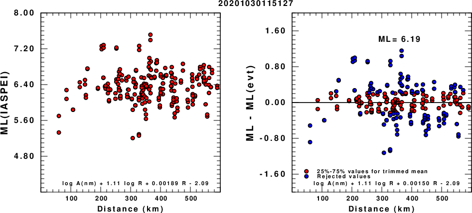
(a) ML computed using the IASPEI formula for Horizontal components; (b) ML residuals computed using a modified IASPEI formula that accounts for path specific attenuation; the values used for the trimmed mean are indicated. The ML relation used for each figure is given at the bottom of each plot.

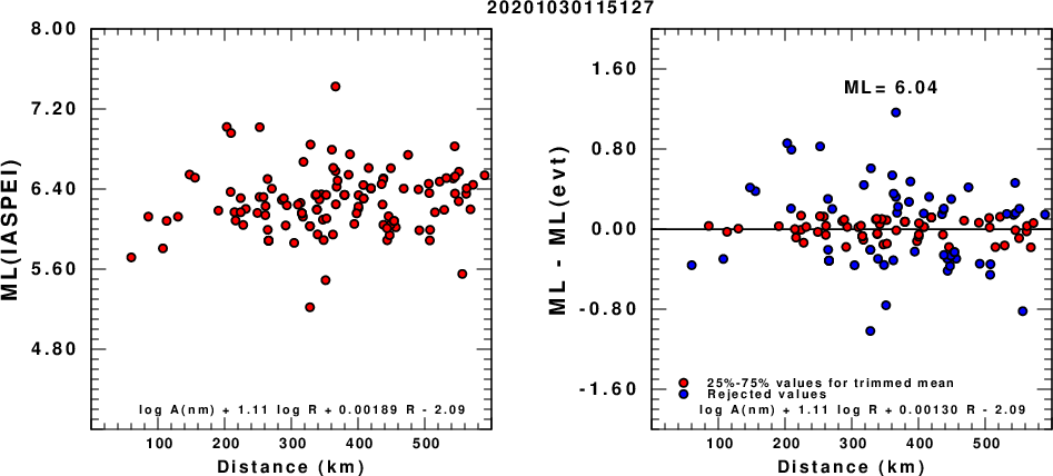
(a) ML computed using the IASPEI formula for Vertical components (research); (b) ML residuals computed using a modified IASPEI formula that accounts for path specific attenuation; the values used for the trimmed mean are indicated. The ML relation used for each figure is given at the bottom of each plot.

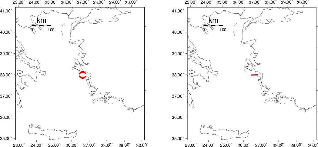
Context

The next figure presents the focal mechanism for this earthquake (red) in the context of other events (blue) in the SLU Moment Tensor Catalog which are within ± 0.5 degrees of the new event. This comparison is shown in the left panel of the figure. The right panel shows the inferred direction of maximum compressive stress and the type of faulting (green is strike-slip, red is normal, blue is thrust; oblique is shown by a combination of colors).

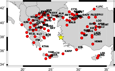
Waveform Inversion

The focal mechanism was determined using broadband seismic waveforms. The location of the event and the and stations used for the waveform inversion are shown in the next figure.

Location of broadband stations used for waveform inversion

The program wvfgrd96 was used with good traces observed at short distance to determine the focal mechanism, depth and seismic moment. This technique requires a high quality signal and well determined velocity model for the Green functions. To the extent that these are the quality data, this type of mechanism should be preferred over the radiation pattern technique which requires the separate step of defining the pressure and tension quadrants and the correct strike.

The observed and predicted traces are filtered using the following gsac commands:

cut o DIST/3.3 -80 o DIST/3.3 +150
rtr
taper w 0.1
hp c 0.01 n 3 
lp c 0.02 n 3

The results of this grid search from 0.5 to 19 km depth are as follow:

           DEPTH  STK   DIP  RAKE   MW    FIT
WVFGRD96    1.0   285    50   -65   6.65 0.4424
WVFGRD96    2.0   110    50   -60   6.69 0.4903
WVFGRD96    3.0   105    50   -70   6.73 0.5395
WVFGRD96    4.0    95    45   -85   6.76 0.5799
WVFGRD96    5.0    95    45   -85   6.79 0.6090
WVFGRD96    6.0    95    45   -85   6.82 0.6243
WVFGRD96    7.0    95    45   -85   6.83 0.6266
WVFGRD96    8.0    95    45   -85   6.85 0.6519
WVFGRD96    9.0    95    45   -85   6.86 0.6407
WVFGRD96   10.0    95    45   -85   6.86 0.6169
WVFGRD96   11.0    95    45   -85   6.86 0.5842
WVFGRD96   12.0    95    45   -85   6.86 0.5442
WVFGRD96   13.0   270    45   -95   6.85 0.4999
WVFGRD96   14.0    95    45   -85   6.84 0.4580
WVFGRD96   15.0   105    45   -70   6.81 0.4190
WVFGRD96   16.0   135    65   -20   6.74 0.4070
WVFGRD96   17.0   135    70   -20   6.73 0.4012
WVFGRD96   18.0   135    70   -20   6.73 0.3962
WVFGRD96   19.0   140    70     5   6.73 0.3930
WVFGRD96   20.0   140    70     5   6.74 0.3917
WVFGRD96   21.0   140    70    10   6.74 0.3896
WVFGRD96   22.0   140    70    10   6.75 0.3892
WVFGRD96   23.0   140    70    15   6.75 0.3897
WVFGRD96   24.0   140    70    15   6.76 0.3909
WVFGRD96   25.0   140    70    15   6.76 0.3924
WVFGRD96   26.0   140    70    15   6.77 0.3938
WVFGRD96   27.0   140    70    15   6.77 0.3955
WVFGRD96   28.0   140    70    15   6.78 0.3974
WVFGRD96   29.0   140    70    20   6.78 0.3999

The best solution is

WVFGRD96    8.0    95    45   -85   6.85 0.6519

The mechanism correspond to the best fit is

Figure 1. Waveform inversion focal mechanism

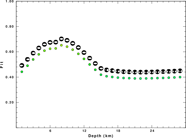
The best fit as a function of depth is given in the following figure:

Figure 2. Depth sensitivity for waveform mechanism

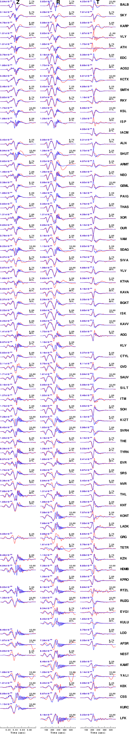
The comparison of the observed and predicted waveforms is given in the next figure. The red traces are the observed and the blue are the predicted. Each observed-predicted component is plotted to the same scale and peak amplitudes are indicated by the numbers to the left of each trace. A pair of numbers is given in black at the right of each predicted traces. The upper number it the time shift required for maximum correlation between the observed and predicted traces. This time shift is required because the synthetics are not computed at exactly the same distance as the observed and because the velocity model used in the predictions may not be perfect. A positive time shift indicates that the prediction is too fast and should be delayed to match the observed trace (shift to the right in this figure). A negative value indicates that the prediction is too slow. The lower number gives the percentage of variance reduction to characterize the individual goodness of fit (100% indicates a perfect fit).

The bandpass filter used in the processing and for the display was

cut o DIST/3.3 -80 o DIST/3.3 +150
rtr
taper w 0.1
hp c 0.01 n 3 
lp c 0.02 n 3

Figure 3. Waveform comparison for selected depth

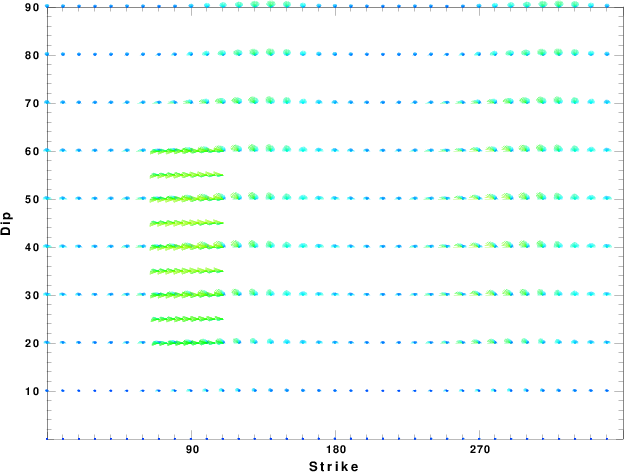
Focal mechanism sensitivity at the preferred depth. The red color indicates a very good fit to thewavefroms. Each solution is plotted as a vector at a given value of strike and dip with the angle of the vector representing the rake angle, measured, with respect to the upward vertical (N) in the figure.

A check on the assumed source location is possible by looking at the time shifts between the observed and predicted traces. The time shifts for waveform matching arise for several reasons:

The origin time and epicentral distance are incorrect
The velocity model used for the inversion is incorrect
The velocity model used to define the P-arrival time is not the same as the velocity model used for the waveform inversion (assuming that the initial trace alignment is based on the P arrival time)

Assuming only a mislocation, the time shifts are fit to a functional form:

 Time_shift = A + B cos Azimuth + C Sin Azimuth

The time shifts for this inversion lead to the next figure:

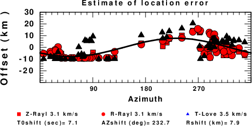
The derived shift in origin time and epicentral coordinates are given at the bottom of the figure.

Discussion

Acknowledgements

Thanks also to the many seismic network operators whose dedication make this effort possible: University of Nevada Reno, University of Alaska, University of Washington, Oregon State University, University of Utah, Montana Bureas of Mines, UC Berkely, Caltech, UC San Diego, Saint Louis University, University of Memphis, Lamont Doherty Earth Observatory, the Iris stations and the Transportable Array of EarthScope.

Velocity Model

The WUS.model used for the waveform synthetic seismograms and for the surface wave eigenfunctions and dispersion is as follows:

MODEL.01
Model after     8 iterations
ISOTROPIC
KGS
FLAT EARTH
1-D
CONSTANT VELOCITY
LINE08
LINE09
LINE10
LINE11
      H(KM)   VP(KM/S)   VS(KM/S) RHO(GM/CC)         QP         QS       ETAP       ETAS      FREFP      FREFS
     1.9000     3.4065     2.0089     2.2150  0.302E-02  0.679E-02   0.00       0.00       1.00       1.00    
     6.1000     5.5445     3.2953     2.6089  0.349E-02  0.784E-02   0.00       0.00       1.00       1.00    
    13.0000     6.2708     3.7396     2.7812  0.212E-02  0.476E-02   0.00       0.00       1.00       1.00    
    19.0000     6.4075     3.7680     2.8223  0.111E-02  0.249E-02   0.00       0.00       1.00       1.00    
     0.0000     7.9000     4.6200     3.2760  0.164E-10  0.370E-10   0.00       0.00       1.00       1.00

Quality Control

Here we tabulate the reasons for not using certain digital data sets

The following stations did not have a valid response files:

Last Changed Tue Nov 24 16:19:32 CST 2020