Computer Programs in Seismology Tutorials - Moment Tensor Sensitivity

Introduction

The determination of earthquake source parameters through moment tensor inversion is a non-linear problem that is affected by many factors which may not be well understood. In the opinion of this author, the association of error to the source parameters may be impossible.

The factors affecting the inversion result are many and include the following:

Earth structure along the path between the source and the seismic station

The objective of the codes for determining source parameters is to model the observed waveforms through a theoretical wave propagation model. The simplest assumption is to assume a single, simple wave propagation model to all observation points. This assumption is never correct, but will be adequate if the focus is on modeling the lower frequency content in the observed waveforms. As one uses higher frequencies, the inability to model 3-D wave propagation, because of the synthetic seismogram codes used and the assumptions about the Earth model, affect the inversion.

Shallow structure beneath the seismic station

Even if the path is relatively simple, a site response may affect the levels of recorded motion.

Seismic instrumentation

Recorded data are noisy because of inherent instrumental noise and installation of the instrument. Such noise can be documented and perhaps mitigated through the selection of the instrumentation and care in installation.

Earth noise

This noise arises through human activity and natural processes related often to atmospheric effects. These noise levels dynamically change on time scales varying from hours, for human activity, to months, for seasonal changes.

The distribution of observations

The actual observations depend on the source depth and source process. One can easily think of distributions of stations whose observations in the presence of noise provide no information for a particular source mechanism.

The purpose of this tutorial is to examine the effect of noise on source inversion results and to determine if goodness of fit parameters can be modeled in a synthetic study. This tutorial will consider a small earthquake in Arkansas, Earthquake of May 22, 2013.

Another aspect of this example is that the ability of determining source parameters as a function of source size may be useful in defining the capabilities of a seismic network.

Modeling noise

The new tool developed for this study is the program sacnoise. Using the USGS Albuquerque Seismc Lab New Low Noise Model (NLNM) and New High Noise Model (NHNM), an acceleration
history in units of meters/s/s (M/S**2) is created as a sac file. The source code and Makefile are given in this distribution in MT_SENSITIVITY/src. The current command syntax is obtained by running the program using the -h flag:

rbh> sacnoise -h
Usage: sacnoise -pval pval -seed seed -dt dt -npts npts 
  Create time series of noise based on ASL NLNM and NHNM models. The output has units of 
     m/s**2   (default)
  The noise level can be adjusted between the low and high noise models with pval
     pval=1   High noise model
     pval=0.5 mid-noise model
     pval=0   Low  noise model
 -dt   dt     (default 1.0) sample interval 
 -npts npts   (default 32768) length of time series 
 -pval pval   (default 0.5) 
 -seed seed   (default 12345) Integer random number seed 
 -h           (default false) online help

To illustrate the usage and the use of the pval parameter, the script DOIT in MT_SENSITIVITY/NOISEPLOTS/ does the following:

Creates 100000 sample long random accelerations for a 0.1 s sample interval using different random number seeds for pval = 0.0, 0.2, 0.3, 0.4 and 1.0. The output of simulation is in the file O.sac.
For each sac file, the program sacpsd is used to compute the power spectrum with tabular output in files named as 0.3.psd, for example.
Finally, all PSD estimates are plotted together using another invocation of sacpsd.

The plot so created is

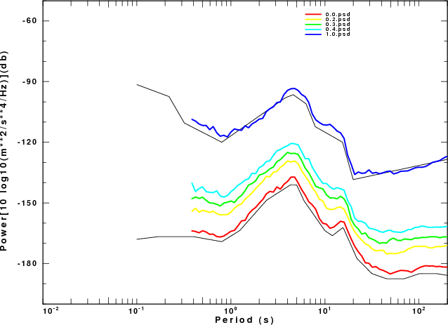
Fig. 1. Comparison of acceleration PSD from sacnoise simulations to the ASL NLNM (lower black curve) and NHNM (upper black curve).

This figure illustrates the use of the pval parameter. The fact that the simulations for pval=0.0 and 1.0 do not lie exactly on the NLNM and NHNM curves is because only one short simulation was performed. To perform realistic modeling, it would be useful to use sacpsd to determine actual noise PSD for stations in a network to guide the choice of the pval. It might also be useful to extend the program to read an actual noise power spectrum for the generation of simulation.

Simulations for source inversion study

The scripts are provided investigate the earthquake of 2013/05/22 17:19:39. The driver script DOIT2 performs 6 simulations as follow:

  Velocity Model   Strike   Dip  Rake  Source Depth   Mw  Noise (pval)  Inversion

        CUS          85      70   -20      2.0       3.38  0.3          CUS.85.70.-20.0020.3.38.0.3/
        CUS          85      70   -20      2.0       3.00  0.3          CUS.85.70.-20.0020.3.00.0.3/
        CUS          85      70   -20      2.0       4.00  0.3          CUS.85.70.-20.0020.4.00.0.3/

        CUS          85      70   -20      2.0       3.00  0.4          CUS.85.70.-20.0020.3.00.0.4/
        CUS          85      70   -20      2.0       3.59  0.4          CUS.85.70.-20.0020.3.50.0.4/
        CUS          85      70   -20      2.0       4.00  0.4          CUS.85.70.-20.0020.4.00.0.4/

    Real Data        85      70   -20      2.0       3.38               20130522171939           [This is not part of the simulation but for reference]

The first simulation uses the Mw determined for the earthquake. The next two vary the Mw. The reason is that we might expect better results for a larger Mw which will provide greater signal-to-noise than for the smaller event. The last three simulations increase the noise level in another examination of the lower limit of applicability of the source inversion. The selected solution for each simulation is given in the files with names such as CUS.85.70.-20.0020.3,38.0.3/HTML.REG/fmdfit.dat.

The goodness of fit parameters for the actual data set and for the six simulations are as follow.

    Directory                 H  STK DIP RAKE  Mw    FIT
20130522171939               2.0  85  70  -20 3.38 0.5615

CUS.85.70.-20.0020.3.38.0.3  2.0  85  70  -20 3.39 0.3885

CUS.85.70.-20.0020.3.00.0.3  2.0 275  80   40 3.09 0.0639
CUS.85.70.-20.0020.4.00.0.3  2.0  85  70  -20 4.00 0.9777

CUS.85.70.-20.0020.3.00.0.4  8.0 130  60   45 3.19 0.0379
CUS.85.70.-20.0020.3.50.0.4  2.0  85  70  -25 3.52 0.3465
CUS.85.70.-20.0020.4.00.0.4  2.0  85  70  -20 4.00 0.9430

We see that the goodness of fit in the simulations depends on the event magnitude, with larger magnitudes giving a better fit, because the increased signal-to-noise ratio. As noise is increased, the fit degrades. Some figures from the detailed presentation of the processing results may help put the results in perspective. We will first compare the goodness of fit plots for the real data set and the first three simulations.

20130522171939	CUS.85.70.-20.0020.3.38.0.3	CUS.85.70.-20.0020.3.00.0.3	CUS.85.70.-20.0020.4.00.0.3

Fig 2a	Fig 2b	Fig 2c	Fig 2d

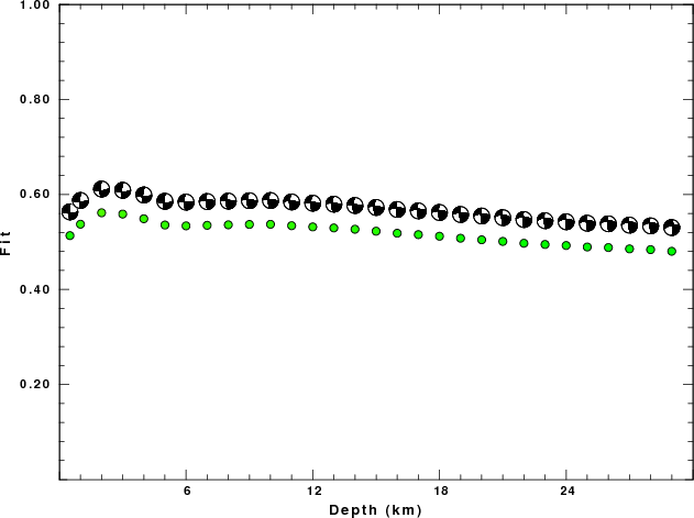
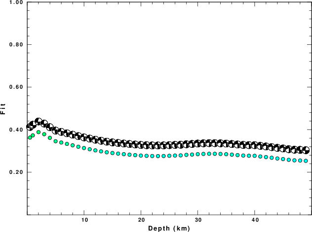
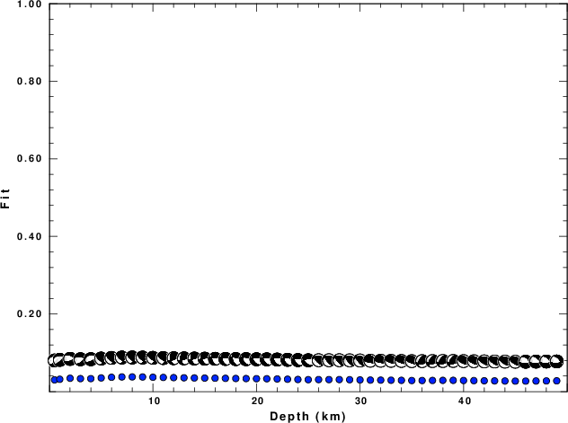
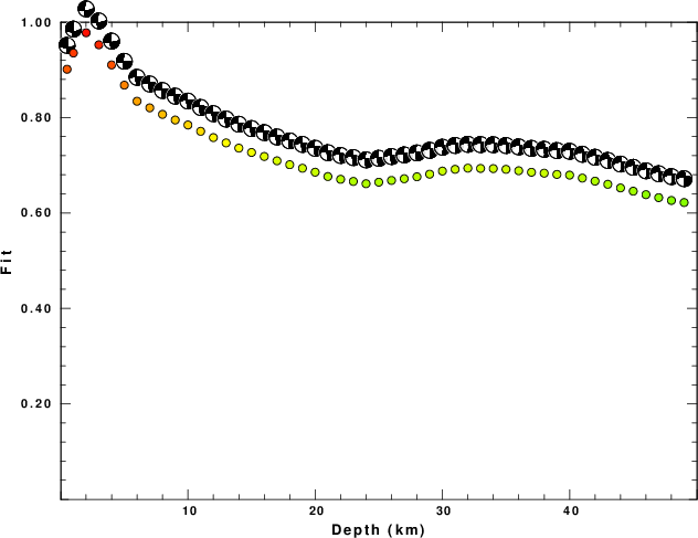
This figure presents the goodness of fit (1.0 is the best fit) as a function of source depth and displays the focal mechanism for the best fit at each depth. First note that the data set for the actual event did not have a well defined best fit. The selected source depth of 2 km is very subtle. The fundamental question is whether the source depth and fault parameters are actually known. The simulation also uses more vertical and radial traces than the real data set.

Interestingly Fig 2b, which is based on synthetics shows a very similar pattern of best fit as a function of depth. In this case the solution is known, which provides the basis for determining if the solution is correct. If the event had been smaller, e.g., Mw=3.0, Fig 2c shows that the fit degrades because of the lower signal-to-noise ratio. The simulation does provide a good estimate of the Mw. Finally, if the event had been larger, Fig 2d, there would have been better control on the depth.

In comparing Fig2b to Fig2d, it seems as if the pattern would be similar if the fit is plotted logarithmically. This is based on the ratio of the best fit value at the 2 km depth to the lower value at a 50 km depth.

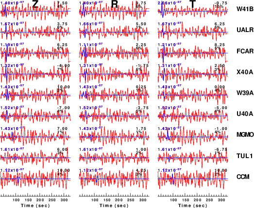
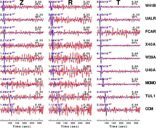
To see the effect of noise consider the waveforms for the pval=0.4 simulations:

CUS.85.70.-20.0020.3.00.0.4	CUS.85.70.-20.0020.3.50.0.4	CUS.85.70.-20.0020.4.00.0.4

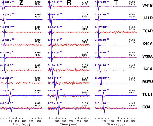Fig. 3a	Fig. 3b	Fig. 3c

Figure 3 compares the waveforms to be modeled (red) to the predicted best fit (blue). The time shift for best fit and reduction in variance are indicated to the right of each trace and the peak filtered velocity (0.02 - 0.10 Hz) is indicated at the left. The actual source inversion used at window width of only 75 seconds whereas the simulation used a window of 270 seconds as a test of the superposition of noise and the clean synthetic.

In comparing the the fits to the observed data to those of the Mw=3.38 pval=0.3 simulations. a similar pattern is seen. For the actual data, many traces were judged too noisy for the source inversion. These were typically the Z and R traces at the larger distances. The simulations indicate that the analyst required a S/N of at least 2 or greater before judging a trace useful.

Perhaps it may be possible to change the grid search used by wvfgrd96 from a single pass to a two-pass process. The second pass would examine the fit to each trace and then automatically down-weight or reject a trace if the fit is less than 20%, or so. The effect of the time window on the fit parameter would have to be investigated.

Annotated processing scripts

The following scripts are provided in this distribution. The annotated scripts are given in the following links:

DOIT2 - this is the driver for simulation 2
DOMKMOD2 - this creates the simulated traces, set up and runs the inversion
DOLL - this utility script estimates the station coordinates from the epicenter and distance and azimuth to each station

Distribution

The processing scripts for this tutorial are in Dist.tgz. Click and save on the link to save this file on your machine. Then unpack using the command

gunzip -c Dist.tgz | tar xvf -

The result of unpacking will be

MT_SENSITIVITY/
               |---0XXXREG/
               |---20130522171939/
               |---CUS.85.70.-20.0020.3.00.0.3/
               |---CUS.85.70.-20.0020.3.00.0.4/
               |---CUS.85.70.-20.0020.3.38.0.3/
               |---CUS.85.70.-20.0020.3.50.0.4/
               |---CUS.85.70.-20.0020.4.00.0.3/
               |---CUS.85.70.-20.0020.4.00.0.4/
               |---DOIT2
               |---DOLL
               |---DOMKMOD2
               |---DOPACK
               |---NOISEPLOTS/
               |---doit2.html
               |---doll.html
               |---domkmod2.html
               |---index.html
               |---src/

After unpacking,

cd MT_SENSITIVITY/src
make

This will compile the program sacnoise. You can then cd .. and run the DOIT2 script