Computer Programs in Seismology Tutorials

Introduction

Distribution

The sample data set and other scripts can be obtained by downloading Dist.tgz and then unpacking with the command

    gunzip -c Dist.tgz | tar xf -
    cd EMPIRICAL_GREEN/DIST

In that folder you will find the following files:

EMPIRICAL_GREEN/DIST/
                    |--/RANDOM4/
                    |          |--DOIT            
                    |          |--MFTDOOVERLAY
                    |          |--PHVDOOVERLAY
                    |          |--DOCLEAN
                    |          |--CUS.mod
                    |
                    |--/EXAMPLE1/
                    |          |--DOSRF
                    |          |--MFTDOOVERLAY
                    |          |--PHVDOOVERLAY
                    |          |--DOCLEAN
                    |          |--SIUCBHZBLOBHZ.WSTK
                    |          |--CUS.mod 
                    |
                    |--/EXAMPLE.GRN/
                               |--CUS.mod
                               |--DOIT
                               |--DOCLEAN

Sac Files

In order to use Sac files that are not created by the Computer Programs in Seismology codes, one must be careful about the following header values:

The O header that sets the origin time must be set
The DIST header which gives epicentral distance in km must be defined .
The USER1 and USER2 headers define the minimum and maximum periods permitted for processing. If uncertain about these values, set each to -12345. using the ch command in sac/gsac. The reason for this specific restriction is that spectral amplitudes should not be used outside the acceptable bandpass region.

If in doubt, look at the header values of the sample cross-correlation in the file SIUCBHZBLOBHZ.WSTK in EMPIRICAL_GREEN/DIST/EXAMPLE1

Theory

The detailed theory is given in MFT.pdf ( updated MAY 31, 2021)

Program Usage

This discussion uses the files in the sub-directory EMPIRICAL_GREEN/DIST/EXAMPLE1. The tutorial on the use of do_mft is here.

Tests

Simulation of a noise field

The critical relationship for the determination of phase velocities is the phase correction applied in Equation (6) of the document MFT.pdf.

Consider the subdirectory EMPIRICAL_GREEN/DIST/RANDOM4. The DOIT script creates a data set consisting of MAXSRC time segments, each of which has 20 source events distributed randomly in a source region 1600 km x 1600 km. Two stations are at coordinates (-200,0) and (200, 0 ) on this grid. The random source coordinates and station coordinates in km are converted to latitude and longitude in order to create a map. For the demonstration script, the values of these parameters are MAXSRC=100 and SUBSOURCE takes the vales 00, 01, ..., 19. A larger value of MAXSRC will yield better results, but the computations will take longer.

The idea is to create MAXSRC time series, representing the different noise segments used with real data. Each of this time series consists of the waveforms or 20 randomly distributed sources. This approach is use to emulate processing of real noise data.

The current DOIT script does the following:

Generates the eigenfunctions and dispersion for the CUS.mod velocity model for a source depth of 0.01 km.
For each time segment (from 0 to MAXSRC -1)

Loop over the subsources, then

Define the spatial coordinates of the subsource
Define a random orientation for a point source applied at the subsource
Compute fundamental mode Green's functions to each of the two stations
Apply the source to create Z, N and E seismograms from the seismograms for the particular force function
Store the Z, E and E seismograms in the sub-directories POS1 and POS2 with a name such as 44.17.Z, which represents the Z component seismogram for time segment 44 and subsource 17. The POS1 and POS2 contain the individual time histories at receiver positions 1 and 2.

Stack the subsource contributions to each seismogram and store appropriately in the sub-directories STACK1 or STACK2 with a name such as 44.Z, which represents the Z component seismogram for the time segment 44.
Cross-correlate the components between the stations and save the result in sub-directory CORR. For example, STACK1/44.Z cross-correlated with STACK2/44.Z will result in CORR/44.Z1Z2. All nine possible cross-correlations are saved, for example, CORR/44.E1E2, CORR/44.E1Z2, CORR/44.N1N2, CORR/44.Z1E2, CORR/44.Z1Z2,
CORR/44.E1N2, CORR/44.N1E2, CORR/44.N1Z2, and CORR/44.Z1N2.

After all time segments are processed, the individual cross-correlations are stacked to form the file Z1Z2, for example. The reversed time series, Z1Z2.rev is computed and as the sum of Z1Z2 and Z1Z2.rev which is called Z1Z2.sym, since it will be symmetric about zero lag. The Z1Z2 and E1E2 will show the Rayleigh wave and the N1N2 will show the Love wave.
Finally, the sac files in POS1 and POS2 are read to create a map.

The question arises as to why this is all done. The objective is to create a model based synthetic data set that can be used to mimic the data sets used in the cross-correlation of ground noise. That processing cross-correlates fixed time windows and then stacks all of the cross-correlations. The use of the synthetic data means that the dispersion is known. Thus the group and phase velocity estimates can be compared to the "true" values. For this example run (realized that your runs will use different random number sequences), the local distribution of sources is shown in the following figure. The yellow stars indicate the source locations and the red dots indicate the receiver positions. Sources are not permitted within 50 km of a receiver to avoid problems with the 1/sqrt(r) geometrical spreading blowing up.

source map

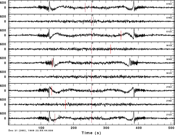
The resulting symmetric traces obtained are

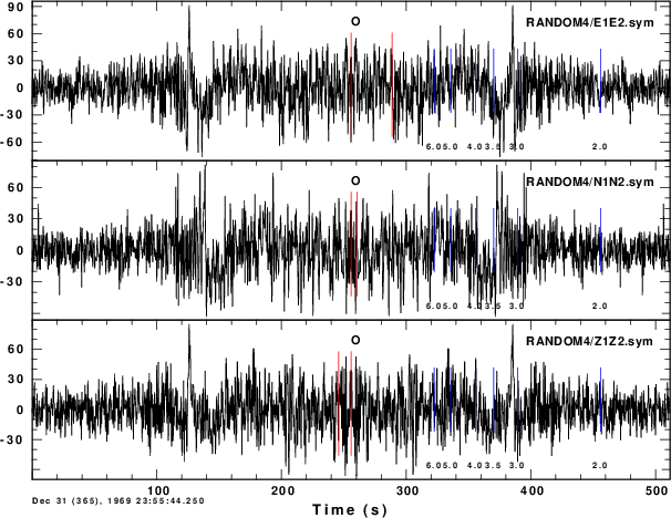
It is seen that there are arrivals with group velocities between 3 and 4 km/s. Since the distributed DOIT script only uses 100 (MAXSRC) time windows, each of which contains the signals of 20 sources, the image will improve if MAXSRC is made larger.

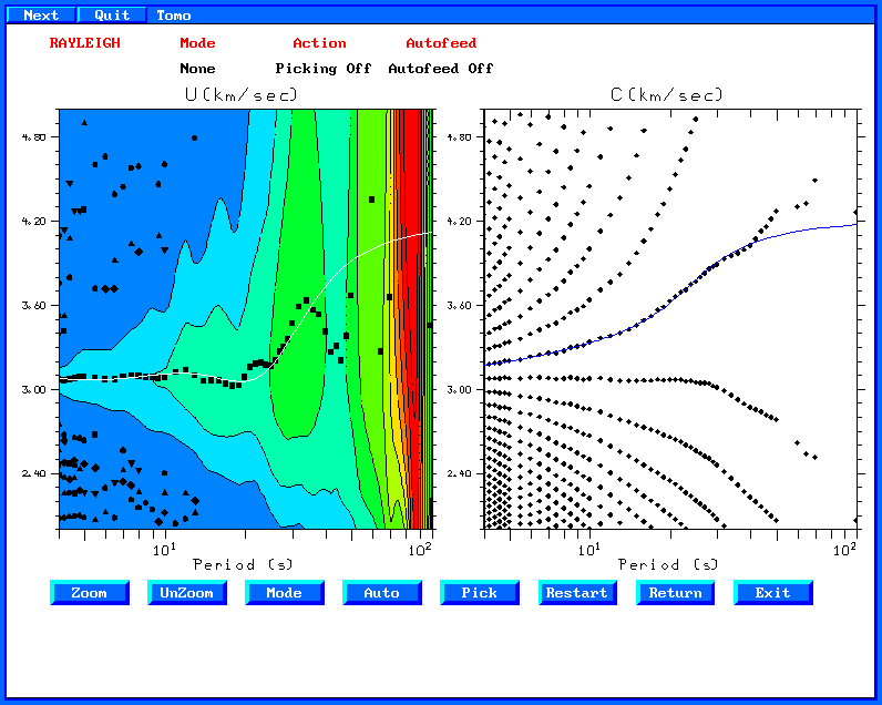
If we now run do_mft in the same directory as the DOIT script, which is important since we have the enigenfunction files slegn96.egn and sregn96.egn and also the scripts required by do_mft, MFTDOOVERLAY and PHVDOOVERLAY to create the theoretical dispersion plots, the command

do_mft -G -IG -T *.sym

leads to the following comparison plots:

groupd velocity

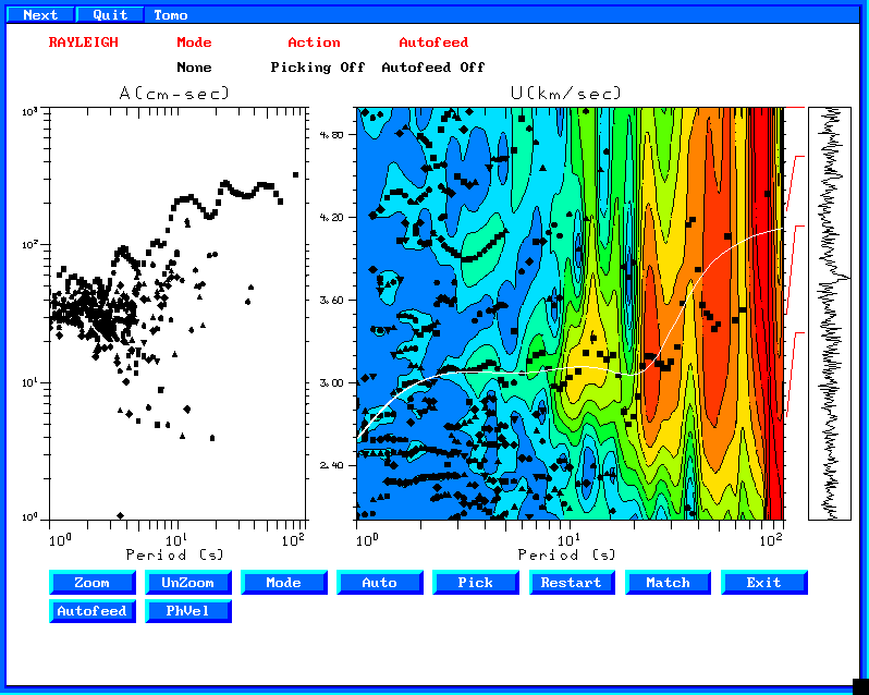
This is the group velocity from the file Z1Z2.sym The white curve is the model predicted group velocity.

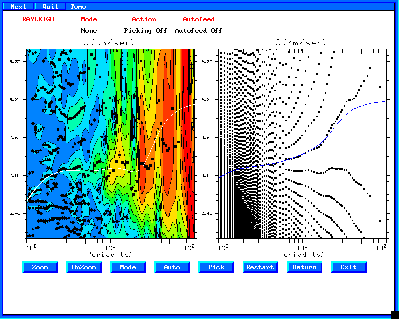
This is the phase velocity panel. Interestingly, there are good phase velocity estimates despite the poor signal.

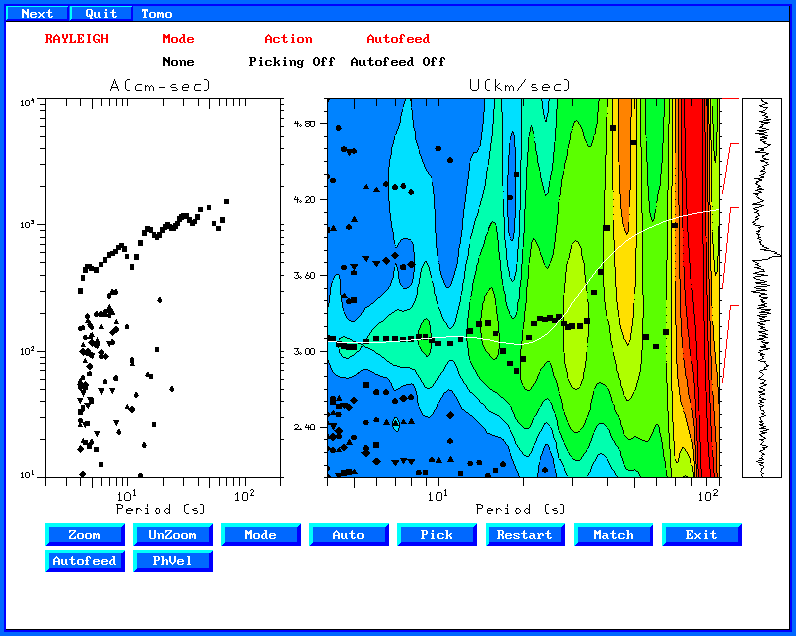
The next figures show a run with MAXSRC=2500. The number of sub-sources for any time window is still 20. The correspond figures are now

group velocity analysis

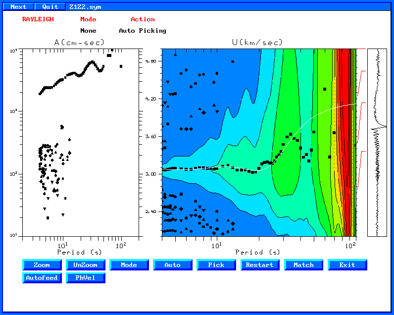
The group velocities are better defined. In addition there is a much better signal to noise ratio on the stacked Z1Z2.sym trace.
The corresponding phase velocity comparison is shown in the next figure.

Here there is superb agreement between the theoretical and experimental phase velocities.

A final set of simulations used MAXSRC=500 and replaced the distribution of point forces at at depth of 0.1 km by a moment tensor source at a depth of 10 km, by changing the -HS 0.1 on the argument of sprep96 to -HS 10, and changing the gsac mt command syntax to a source with strike 0, dip 80n and rake 10, e.g.,

#mt to ZNE AZ ${AZ2} BAZ ${BAZ2} FN $FN FE $FE FD $FD FILE $B
mt to ZNE AZ ${AZ2} BAZ ${BAZ2} STK 0 DIP 80 RAKE 10 MW 2  FILE $B

Running do_mft with the same arguments, leads to the following images:

EQ group velocity

and

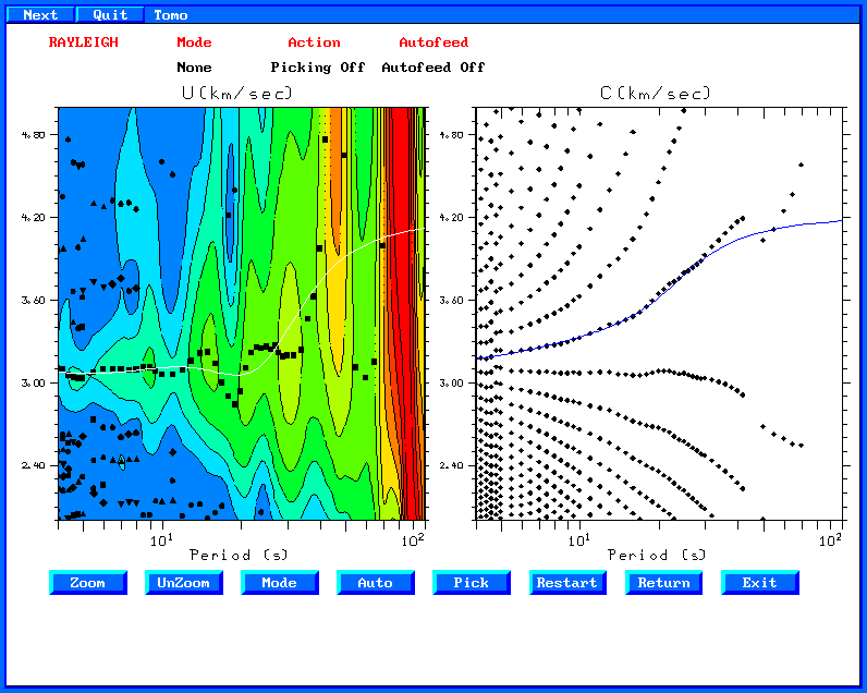
As expected by theory, the distribution of earthquakes sources leads to the same results.

One should be careful, in that one might be tempted to use the Z1E2.sym cross-correlation. Theory says that the Rayleigh wave in the Z1E2 is 90 degrees out of phase with the Z1Z2 time series. Although both will have the same group velocity, the phase velocity from Z1E2 will not be correct since do_mft (sacmft96) does not account for the extra 90 degree phase difference.

Since the logic behind the scripts works, it is now possible to consider the effect of less-uniform source distribution on the stacks and the dispersion analysis.

Other cross-correlations

In running the script for MAXSRC=2500 and 20 subsources consisting of randomly directed forces, 9 inter-component cross-correlations can be computed. The previous discussion focused on the E1E2, N1N2 and Z1Z2. The next figure displays all nine.

all none cross correlations
These are displayed with the gsac command ylim all so that the same amplitude scale is used for each. As expected for a uniform medium, the Z1N2, N1Z2, N1E2 and E1N2 cross-correlations are very small. From the theoretical development of Wapenaar (2004), we would expect the Z1N2, for example, to be related to the wavefield at the second sensor in the +N direction (negative transverse) due to a point upward vertical force at the first. Theoretically zero transverse motion is generated by this symmetric vertical source. The N1E2, the radial motion generated by a transverse source should also be zero because of the radiation pattern when the observation point is in a direction perpendicular ot the direction of the horizontal force.

Generating the proper synthetic

To test an inverted velocity model, synthetics can be generated for comparison to the empirical Greens functions. The waveforms will not be similar because of a different frequency content. Both can be whitened for comparison and then similarly bandpass filtered.

Consider the DOIT script in DIST/EXAMPLE.GRN. Green's functions are computed for the fundamental mode surface wave for a source depth of 0.01 km and a receiver at the surface. The gsac command mt is used to make three component synthetics for a vertical force, Z1Z2 Z1N2 Z1E2, a radially directed horizontal force, E1Z2 E1N2 E1E2, and a transversely directed force, N1Z2 N1N2 N1E2.

Next given the Z1Z2, etc files in EXAMPLE.GRN and the symmetric empirical Greens functions in RANDOM4, run the following commands:

for i in Z1Z2 N1N2 E1E2
do
gsac << EOF
r EXAMPLE.GRN/$i RANDOM4/$i.sym
whiten freqlimits 0.01 0.02 0.25 0.5
w $i.G $i.E
q
EOF
done

#####
#    make a plot
#####
gsac << EOF
r E* N* Z*
xlim o 80 o 180
ylim all
fileid name
bg plt
p
q
EOF

plotnps -BGFILL -F7 -W10 -EPS -K < P001.PLT > t.eps
convert -trim t.eps EMPGRN.png

The whiten command with the zero-phase bandpass filter gives the same amplitude spectrum to both. The resultant plot is

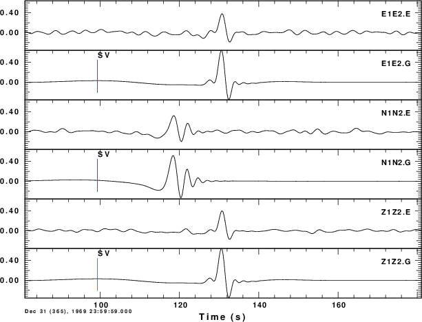comaprison between synthetic and empirical Green

The

The .G are from the synthetics and the >E are from the cross-correlation. The waveform comparison is very good. The difference in absolute amplitude is no problem.
The demonstrates that synthetics can be generated to mimic the noise cross-correlation results. This may be valuable to understand the limitations of the group and phase velocity analysis, expecially at very short distance.

References

Bensen, G. D., M. H. Ritwoller, M. P. Barmin, A. L. Levshin, F. Lin, M. P. Moschetti, N. M. Shapiro and Y. Yang (2007). Processing seismic ambient noise data to obtain reliable broad-band surface wave dispersion measureements, Geophys. J. Int. 169, 1239-1260. doi: 10.1111/j.1365-246X.2007.03374.x

Herrmann, R. B. (1973). Some aspects of band-pass filtering of surface waves, Bull. Seism. Soc. Am. 63, 663-671.

Lin, Fan-Chi and Moschetti, Morgan P. and Ritzwoller, Michael H. (2008). Surface wave tomography of the western United States from ambient seismic noise: {Rayleigh} and Love wave phase velocity maps, Geophys. J. Int. 173, 2810298, doi 10.1111/j.1365-246X.2008.03720.x

Snieder, R. (2004). Extracting the Green's function from the correlation of coda waves: A derivation based on stationary phase, Physical. Rev E 69, 046610-1,10

Wapenaar, K. (2004). Retrieving the elastodynamic Greens function of an arbitrary inhomogeneous medium by cross correlation, Phys. Rev. Lettrs. 93, 254301-1 - 254301-4.

last changed November 8, 2013