do_mft sample run

Introduction

The files for this example are in EMPIRICAL/GREEN/EXAMPLE1. To perform the processing, you will have to set your shell PATH variable to point to the current direction, e.g., in bash

export PATH=:.:$PATH

You will find the following files in this directory:

SIUCBHZBLOBHZ.WSTK - This is a typical result of noise cross-correlation
DOSRF - This creates the eigenfunctions required to give the theoretical dispersion
MFTDOOVERLAY
PHVDOOVERLAY - These are sample scripts for overlaying a dispersion curve on the results of the processing.
CUS.mod - Velocity model to provide dispersion curves
DOCLEAN - This cleans up after a processing run

The two scripts MFTDOOVERLAY and PHVDOOVERLAY can be modified to use results of your tomography to provide reference dispersion curves.

Note that if you do not have an Intel/AMD computer, e.g., a SPARC you will have to get the correct byte order in the Sac file, but entering the commands

     saccvt -I < SIUCBHZBLOBHZ.WSTK > t
     mv t SIUCBHZBLOBHZ.WSTK

Starting the program

The program do_mft options can be seen by running the command

do_mft -h
Usage: do_mft [-Nnumberperpage] [-G] [-T] [-11MIN min11] [-11MAX max11] [-DMIN dmin] [-DMAX dmax] sacfiles
  e.g.:  do_mft -N2 -G -T *Z
  -Nnumberperpage  (default 10) number of file menu items per page
        this option is useful when using a slow connection since writing 
        a complete menu takes time
  -G              (default off) The default dispersion file name is of the form 
        StationComponent.dsp, e.g., SLMBHZ.dsp 
        When working with ground-noise crosscorrelation for interstation Green functions, the
        naming is Station1Component1Station2Component2.dsp , e.g., SLMBHZFVMBHZ.dsp
  -T              (default off)  run script MFTDOOVERLAY
  -11MIN min11 
  -11MAX max11 
  -DMIN  dmin 
  -DMAX  dmax 
   These options control the selection of the files for MFT
   analysis. The first two use the number in the IHDR11 field,
   which is the number of waveforms stacked for cross-correlation 
   of ground noise. The last two select the distances 
  -IG             (default false)  Inter-station phase velocity from cross-correlation 
  -h              (default false)  Usage

Some of these options are useful when working with the cross-correlation of ground noise. If there are N stations, then shere are N(N-1)/2 station pairs. When working with TA data, the number of station pairs is huge for manual anlysis using do_mft. The -DMIN and -DMAX flags permit the selection of a range of distances. The IHDR11 field is created by the gsac stack command set this parameter with the number of trces stacked. The chances of a useful cross-correlation should be better if the number of traces stacked is larger.

The -T option permits the display of the Tomo buttons of do_mft. On pressing these buttons, the scripts MFTDOOVERLAY or PHVDOOVERLAY are executed.

The -IG option permits the interctive phase velocity analysis.

Example

Before running this example, go to the example directory:

cd EMPIRICAL_GREEN/DIST/EXAMPLE1

Now create the eigenfunctions which are used to provide the theoretical dispersion curves:

DOSRF

Start the example by entering

do_mft -G -IG -T *.WSTK

The processing example follows:

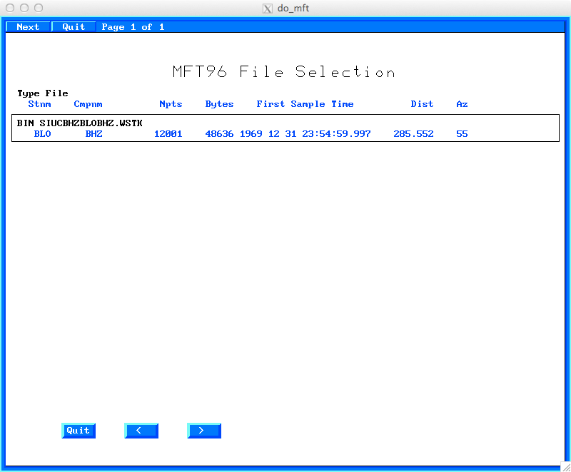
Place the mouse cursor on the trace of interest, and click. You will then see the next page.

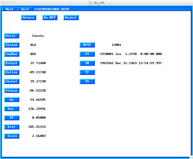
Click on "Units" to seelct the physical units of the trace. For quantitative studies using spectral amplitudes, e.g., to determine earthquake source parameters, the proper physical unit must be used. For my source inversion processing, the traces always represent ground motion in m/sec.

When working with empirical Green's functions from noise cross-correlation, select "Counts" as the unit. For such studies we are interested in the dispersion and not the spectral amplitude.

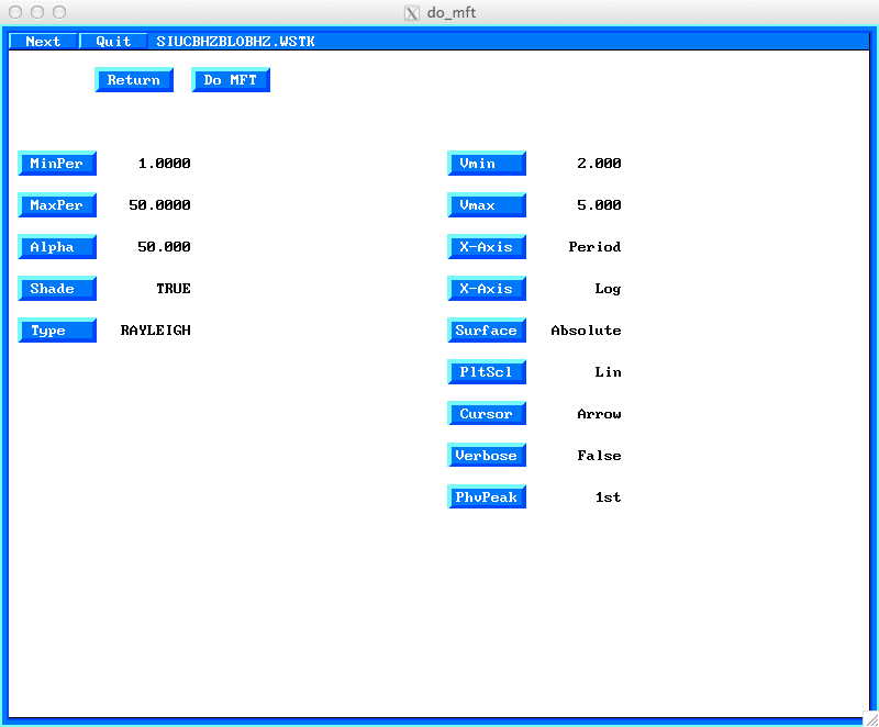
After clicking on the "Do MFT" at the top of the page, we get a page for specifying parameters for the program sacmft96 which does the work. Recall that the purpose of do_mft is to graphically select the output from sacmft.

In this menu, I have have selected the period range of 1.0 to 50.0 seconds and identified the wave type as "Rayleigh" by clicking on the buttons and selecting a value. The "PhvPeak" menu item appears only because of the "-IG" flag used when starting do_mft. Clicking on "PhvPeak" will either give the message "1st" or "1st & 2nd".

The purpose of this is the following. The multiple filter analysis consists of applying a narrow band pass filter to the waveform. Up to 10 envelope peaks are determined. This may be useful to follow a mode in the presence of other signal. However since each envelope peak can be used to estimate a phase velocity, and because each phase velocity estimate has other possible values because of the N2π phase ambiguity, the phase velocity display can be very cluttered and difficult to use. To keep that clean, and assumoing that the larger spectral amplitudes (envelope peak values) will have better determined phase velocities, this menu restricts output to the largest or largest two envelope peaks.

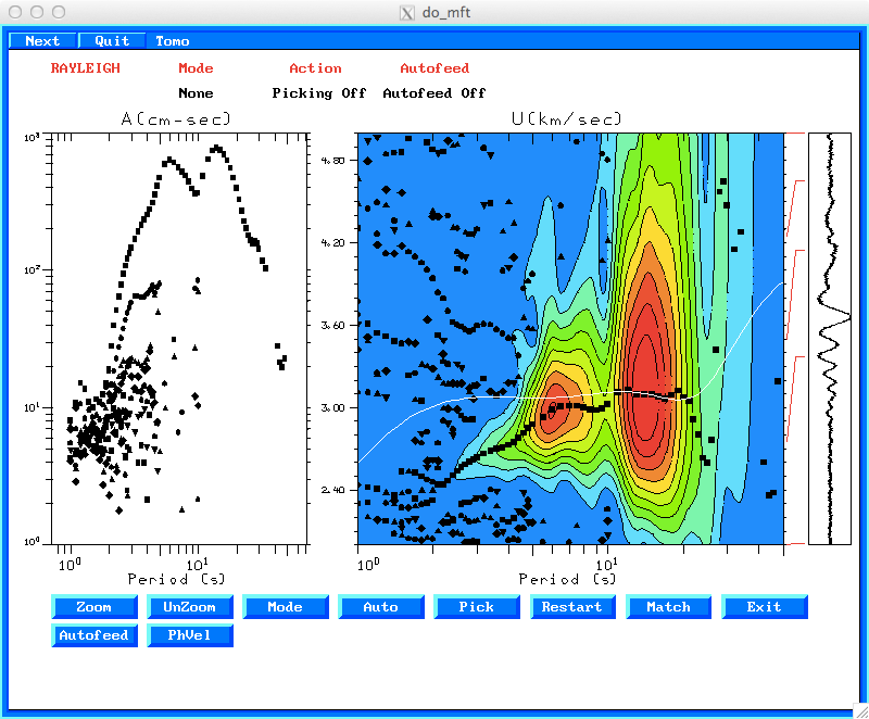
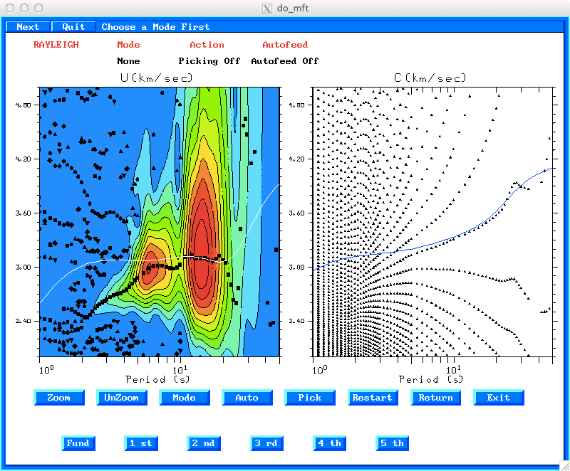
Upon clicking on "DoMFT", the program sacmft96 is run, and the following display is shown. At the bottom of that display will be a button "Tomo" because of the "-T" flag when do_mft was started. On clicking "Tomo" , a dispersion curve in white (note this only works when the background is shaded) is displayed and the "Tomo" button is removed.

This path between two stations of the Saint Louis University component of the New Madrid Seismic Network (NM) goes through part of the Illinois Basin which has deep sections of paleozoic strata.
This is the reason that the observed dispersion at short periods lies beneath the model prediction.

If we now click the "PhVel" button a new image appears. The group velocity overlay picture is reproduced from the previoous display. If we again click the "Tomo" button, the model predicted phase velocities are displayed together with the possible phase velocities. The "Tomo" button is now displayed. The purpose of the overlay is to use the prior knowledge of the predicted curve, which is based on a reasonable velocity model for the area, to resolve the N2π phase ambiguity.

"Autofeed" is set the processing state, so that the 2nd and 3rd menus do not appear. This assumes that one is comfortable with the processing parameters. The effect is that fewer mouse movements and clicks are required. This is very important when processing many, many waveforms.

Now click on "Auto" which brings up a menu to define the mode.

After the mode is selected, the top of the figure will display the parameters. "Auto Picking" means that a rubber band can be used to select a group of points closest to the line.
The selected points are plotted in red in the next figure. As phase velocity values are selected, the corresponding group velocity values are highlighted. This provides confidence that the proper mode is selected.

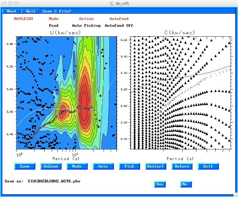
One can also use the "Zoom" buttom to focus in on part of the plot. Click on "Zoom" and then click on a point in the right figure and move the mouse. You will see a box open. Click again and the region will be expanded. You will also see the selected points. You can now select a few more, here shown in red.

When done seleting, click "Exit" you will asked whether to save the picks. You do not have to save the picks if you do not believe them. In this case we will save them. The file created used the original file name and appends a .phv, e.g., SIUCBHZBLOBHZ.WSTK.phv to identify the pahgse velocity selection. The use of the file name occurs because the "-G" flag ws used in invoking do_mft.

You are now returned to to the group velocity selection page. We again use the "Auto" command, identify the "Fund" mode, and select the dispersion. The corresponding spectral amplitudes are colored. For earthquake studies, the shape of the amplitude spectrum has some theoretical expectations as a function of period. This knowledge can be used to define the range of acceptable periods.

On clicking the "Exit" the user is asked whether to save the results in the file SIUCBHZBLOBHZ.WSTK.dsp. We will respond "Yes" to this question. The control returns to the first page display that lists the file names.

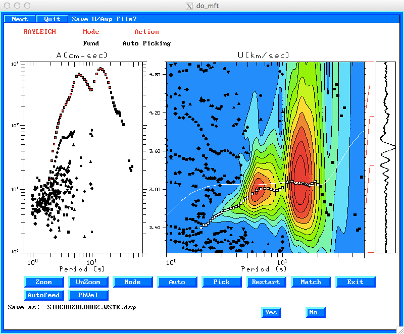
Since this discussion focused on the dispersion estimates, there was no discussion of the "Match" button which uses the group velocity picks to phase match filter the seismogram to isolate a mode.

Output formats

The two files SIUBHZBLOBHZ.WSTK.dsp and SIUCBHZBLOBHZ.WSTK.phv are very similar. Both have many columns. The group velocity outpu is identified by the initial MFT96 and the pahse velocity by the initial PHV96. The SIUCBHZBLOBHZ.WSTK.phv file has three additional columns

MFT96 R U  0          20     3.07357     0.66166   285.5515   54.7  3.9580e+02 37.714802 -89.217400 39.171902 -86.522202 0 1 19.309999 COMMENT: BLO BHZ 1970 1 0 0
MFT96 R U  0          19     3.12174     0.64843   285.5515   54.7  4.7050e+02 37.714802 -89.217400 39.171902 -86.522202 0 1 18.469999 COMMENT: BLO BHZ 1970 1 0 0

         
PHV96 R C  0          20     3.57038     0.00100   285.5515   54.7  3.9580e+02 37.714802 -89.217400 39.171902 -86.522202 0 1 19.309999 COMMENT: BLO BHZ 1970 1 0 0 -1.436470 3.073600 -1
PHV96 R C  0          19     3.54042     0.00100   285.5515   54.7  4.7050e+02 37.714802 -89.217400 39.171902 -86.522202 0 1 18.469999 COMMENT: BLO BHZ 1970 1 0 0 -1.920620 3.121700 -1

The columns are as follow:

Column     Value
1                Type of file, either MFT96 or PHV96
2                Wave type: R for Rayleigh and L for Love
3                Dispersion type: C for phase velocity and U for group velocity
4                Mode: 0 represents the fundamental mode
5                Filter period, T, in seconds
6                Dispersion value, either group or phase
7                Error in dispersion. This is just a place holder since there is no way to estimate an error from a single trace. The group velocity error is determined from the ratio of the filter period to travel time
8                Distance in km
9                Azimuth from the source to the receiver
10              Spectral amplitude. If an initial physical unit were given on Page 2, e.g., m/s, m, this would be the spectral amplitude in cm-sec.
11              Epicenter latitude
12              Epicenter longitude
13              Station latitude
14              Station longitude
15              control flag
16              control flag
17              Instantaneous period if this is preferred. This differs from the ilter period because the signal spectram is not flat.
18              Comment:    keyword
19              Station
20              Component
21              Year
22              Day of year
23              Hour
24              Minute    - these identify the event origin time


For the PHV96 file, there are three additional columns:

25              Phase - this is the phase term
26              This is the N in N2π. The phase velocity, c, is obtained from 1/c = [ -Phase - π/4 + π/2 + ωr/U + N2π] / ( ωr ) where U is the group velocity, r is the epicentral distance and ω = 2π/T. I do not use the instantaneous period.

The purpose of this length format is to provide spectral amplitudes, distance and azimuth for a study of the surface-wave spectra,
to provide information for surface-wave tomography, e.g., the dispersion value and the coordinates of the source and receiver, and finally
dispersion values for use with surf96 or joint96 or shallow96.   If we enter the command

MFTSRF *.dsp *.phv

we get the dispersion in the surf96 format, e.g.,

SURF96 R U X 0 20 3.07357 0.66166
SURF96 R U X 0 19 3.12174 0.64843
SURF96 R U X 0 18 3.09009 0.60191
SURF96 R U X 0 17 3.06323 0.55863
SURF96 R U X 0 16 3.07775 0.53076
SURF96 R U X 0 15 3.09434 0.50297
SURF96 R U X 0 14 3.09599 0.46994
SURF96 R U X 0 13 3.09202 0.43525
         .............
SURF96 R C X 0 2.4 2.85734 0.00100
SURF96 R C X 0 2.3 2.83691 0.00100
SURF96 R C X 0 2.2 2.81739 0.00100
SURF96 R C X 0 2.1 2.79642 0.00100
SURF96 R C X 0 2 2.75870 0.00100
SURF96 R C X 0 1.9 2.73027 0.00100
SURF96 R C X 0 1.8 2.70266 0.00100