WUS 25 km x 25 km tomography

Western US tomography

Interactive map to view dispersion curves for Western US 25 km x 25 km grid (Last update January 18, 2019)

GIF animations

To appreciate the regional variation in dispersion, the images at discrete periods are connected in a GIF animation. In the following figures, the color scale corresponds to a ± 20%. However the original data are clipped at ± 10% in order to permit the eye to focus on small changes. The animations also serve to illustrate the completeness of the tomographic coverage. The tomographic inversion code preserved the sum of ray paths through each inversion cell. If the sum is less than 10 km, the cell dispersion in the cell is not plotted since there is no data to constrain the dispersion in that cell other than the smoothness criteria.

In the plots, the color red indicates a value slower than average, and blue faster than average. The percentages are indicated in the scaling bar.

The group velocity results are the result of earthquake and ambient noise data sets. At the longer periods, where noise data are sparse, one may see the individual ray paths between an earthquake and a station. The inversion uses only sources and receivers within the mapped area.

More experimentation is required to improve the visual presentation so that detailed information is properly conveyed.

Velocity model selection

The surface wave tomography results are an important constraint on velocity models for the purpose of inverting for Earth structure at a specific coordinate. Another important use is the selection of a velocity model to use for location or for regional moment tensor inversion. This figure shows the current tomography results for this coordinate. The results include the SLU and the LDEO values. For each panel, e.g., Love or Rayleigh, phase or group velocity, the theoretical dispersion for the CUS and WUS velocity models are also displayed.

At this coordinate, it is obvious that the WUS model fits the observed dispersion better than the CUS model. Note that these models are crustal models, and thus fail at the very long periods.

The models are tabulated in Computer Programs in Seismology Model96 format at (/eqc/eqc_mt/MECH.NA/MECHFIG/mech.html) .

Clicking on a coordinate to select a velocity model is tedious. To permit a more rapid assessment, the next figure was produced.

Selection among standard models
The purpose here is to indicate which of the three models is best for th region. Investigation of performance of CRUST1.0
The purpose here is to compare the performance of CRUST1.0 compared tot he standard models. The difference between the two models incidates where CRUST1.0 offers a better fit to the disperison. Note that at each position where CRUST1.0 is best, the CRUST1.0 is a unique velocity model and not a generic model such as the three others. Discussion

Map showing preferred velocity model. The colors indicate the preferred velocity model, and the size of the symbol indicates the degree of agreement between the observed dispersion values (L/R and c/U) and the model prediction. The size of the symbol indicates the RMS error in between the observed and predicted dispersion. A Large symbol is preferred.
The metric uses is not completely consistent since the tomopgraphy results differ for each cell in terms of the number of periods used.
In regions at color boundaries, some judgement is required.
Another caveat is that these are models for a specific coordinate or source region. Regional Moment Tensor inversion can use data out to 600 km for larger events (M=4.5) and longer periods, but could also use the specific local model for smaller earthquakes with just close-in data.
The problem of locating earthquakes again depends on the distance range of observations.
This figure is a crude visualization of a 3-D model with emphasis on the variation of the upper half of the crust.


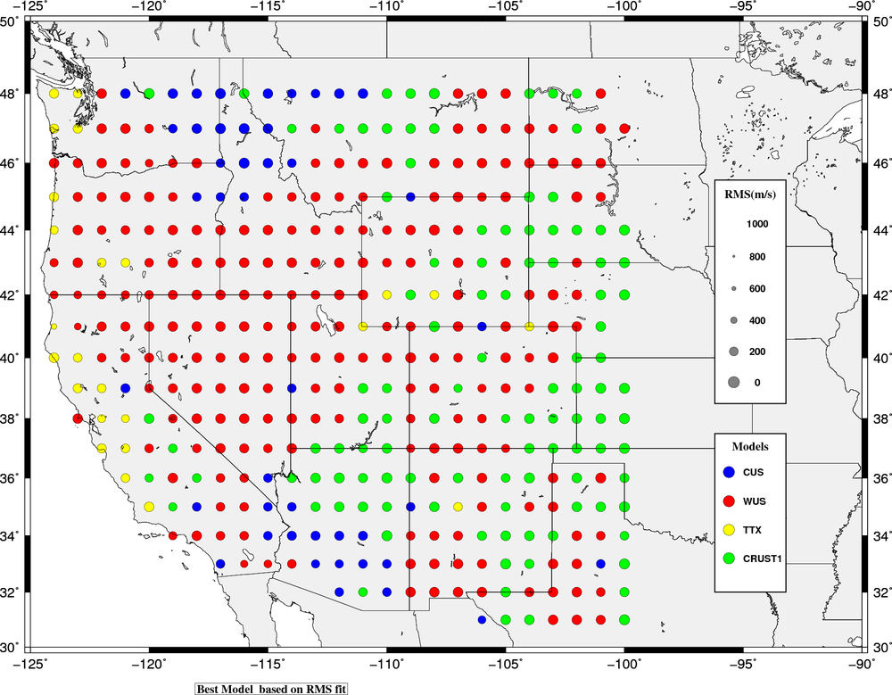
Selection among standard models The purpose here is to indicate which of the three models is best for th region.	Investigation of performance of CRUST1.0 The purpose here is to compare the performance of CRUST1.0 compared tot he standard models. The difference between the two models incidates where CRUST1.0 offers a better fit to the disperison. Note that at each position where CRUST1.0 is best, the CRUST1.0 is a unique velocity model and not a generic model such as the three others.	Discussion
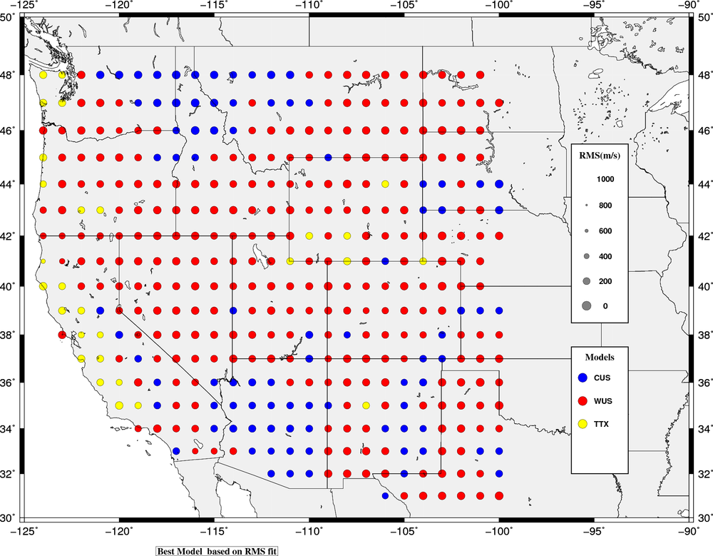		Map showing preferred velocity model. The colors indicate the preferred velocity model, and the size of the symbol indicates the degree of agreement between the observed dispersion values (L/R and c/U) and the model prediction. The size of the symbol indicates the RMS error in between the observed and predicted dispersion. A Large symbol is preferred. The metric uses is not completely consistent since the tomopgraphy results differ for each cell in terms of the number of periods used. In regions at color boundaries, some judgement is required. Another caveat is that these are models for a specific coordinate or source region. Regional Moment Tensor inversion can use data out to 600 km for larger events (M=4.5) and longer periods, but could also use the specific local model for smaller earthquakes with just close-in data. The problem of locating earthquakes again depends on the distance range of observations. This figure is a crude visualization of a 3-D model with emphasis on the variation of the upper half of the crust.

Model performance

The next set of figures shows how well each model fits the dispersion. In this figure the size of the symbol and the color indicate the goodness of fit: red and large indicates a good fit.

CUS Model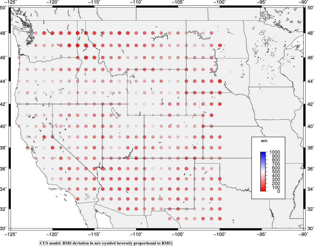	WUS Model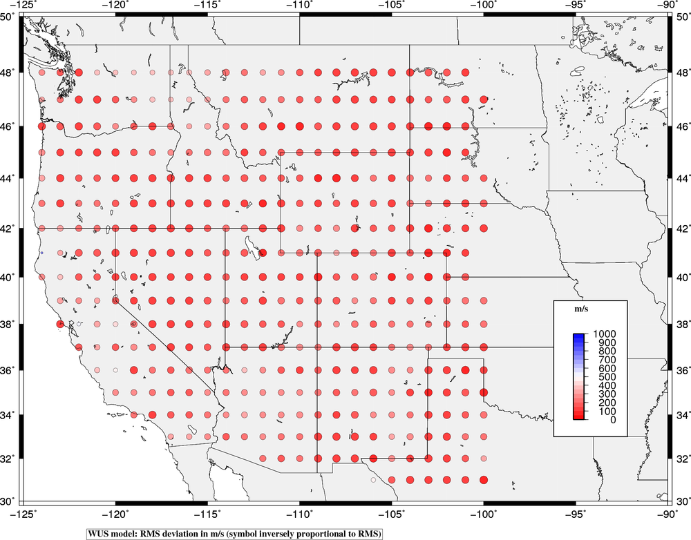
TTX Model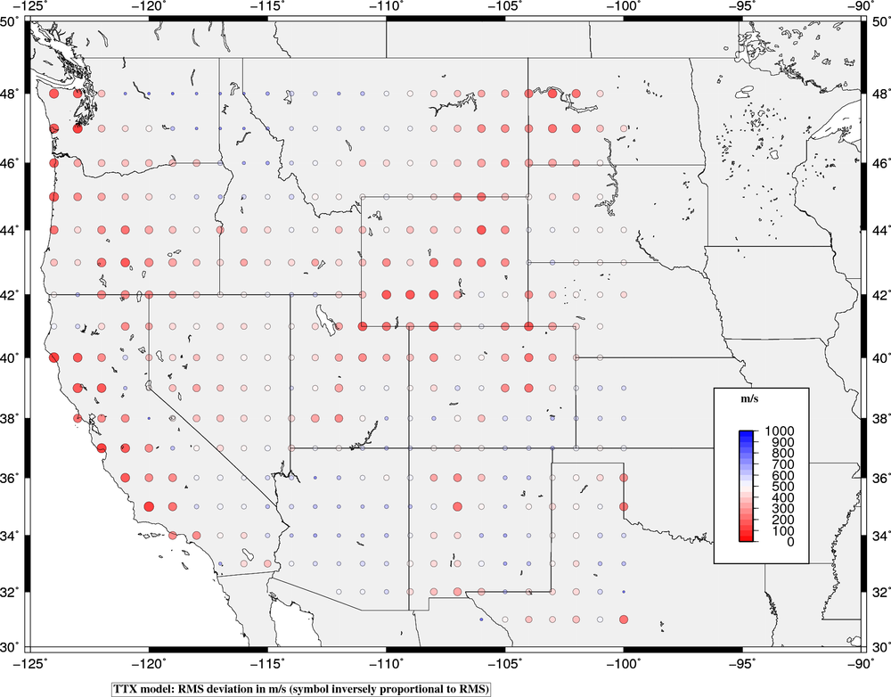	CRUST1 Model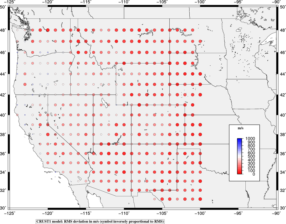