This study compiled a significant number of observations that are electronically available for download at the download sites mentioned in the paper. However this electronic supplement contains supporting material that would be too extensive or impossible to include in the paper itself.
The tomographic inversions created maps for each period and wave type for each of the regions. These maps were used to review the individual inversion results to check for spatial consistence and areas where there may be problems with individual observations. Since there about 70 periods considered, this led to 280 maps for each of the Alaskan and Continuous U.S. studies because the study involved Rayleigh and Love waves as well as group and phase velocities. This large number of images could not be quickly absorbed individually. Instead MP4 movies were created for each set of 70 images.
The movies serve a number of purposes. First spatial outliers are easily identified. Second the completeness of the data sets as a function of period is easily appreciated. Finally since one can say that the depth of penetration of the surface wave is proportional to period, the displays provide a sense of the lateral variation of earth structure with depth.
The following links give the maps for a given data type as a function of period. The shading shows the percent variation of the dispersion value with red indicating slower and blue faster than average. The large number to the bottom right is the period of the frame. Since surface wave penetration is on the order of a fraction of a wavelength, the period shown can be used as a surrogate for depth in kilometers.
The legend at the bottom of each frame indicates the period, average and extremal velocity as well as number of observations in the inversion. Finally the scale at the left relates the color palette to the percent of deviation from the mean.
The presentation of Love wave group velocities at periods between 10 and 15 seconds indicates a very high velocity patch within a broad low velocity region at (29N, 97W). This is strange and most likely is the effect of a bad set of data. At longer periods the results show a random pattern which reflects the paucity of observations.
These mp4 movies display on the Chrome, Firefox, Safari and Edge web browsers.
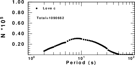
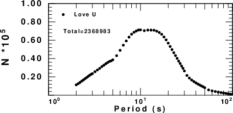
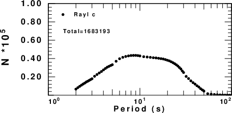
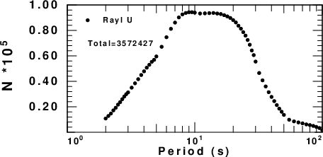
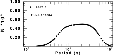
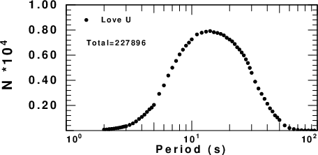
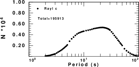
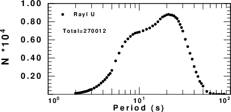
The tomography data sets consisted of group and phase velocities for Love and Rayleigh waves which were obtained from earthquake recordings and ambient noise cross-correlations. The earthquake data provided only group velocities while the ambient noise processing provided phase velocities in addition. Since earthquake dispersion values are affected by location and origin time uncertainty, the inversion of the combined data set duplicated the ambient noise dispersion values to weight then more. The tabulations below show histograms of the number of observations as a function of period.
This data set consisted of 1,474,719 dispersion values from 213 earthquakes and 5,874,129 from ambient noise cross-correlations.
This data set consisted of 4,741 dispersion values from 8 earthquakes and 878,756 from ambient noise cross-correlations.
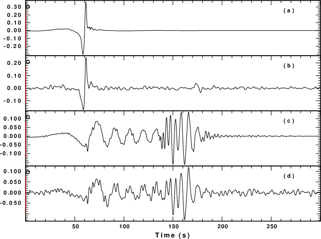
Modeling followed the procedure described in the Compute Programs in Seismology Tutorial Update to do_mft for the determination of phase velocities from empirical Green's functions. Figure 7 - 9 presented a study of the effect of crustal structure on the Rayleigh wave. These figures focus on the cross-correlations between the transverse components which give the Love wave.
|
| Comparison of the multimode synthetic to the empirical Green's functions. All waveforms were first whitened between 0.02 and 1 Hz, and then low-pass filtered with a 3 pole Butterworth filter at 0.2 Hz. The top two traces, (a) and (b), are for the Rock model and the last two, (c) and (d), are for the Deep sediment model. The epicentral distance is 200 km. Traces (a) and (c) are the point horizontal force Green’s functions for the velocity model while traces (b) and (d) are the first derivatives of the ambient noise cross-correlation of the transverse components. The time scale gives the travel time. |
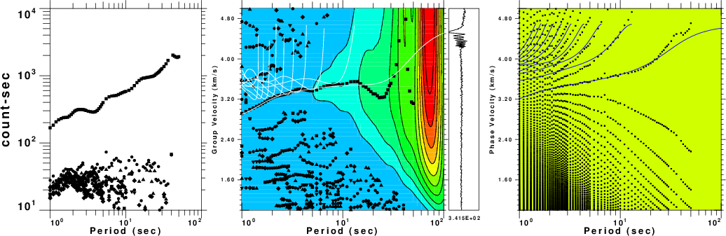 |
| Determination of Love wave group (center) and phase (right) velocities for the Rock model with a station separation of 200 km. The theoretical multimode group (white) and phase (black) velocity curves for the model are also plotted. The color shading in the group velocity plot is scaled to the envelope amplitude at each filter period, with amplitude increasing from blue to red. At each period in the group velocity display, the group velocity corresponding to of the largest envelope peaks (up to 10) are plotted. |
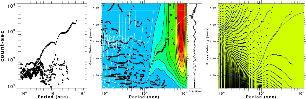 |
| Determination of Love wave group (left) and phase (right) velocities for the Deep sediment model with a station separation of 200 km. |
This simulation indicates that the Love wave dispersion could be made at short periods. However the more rapid roll-off of spectral amplitudes at shorter periods may preclude the such a determination with real data.