 >/td>
>/td>You are permitted to use these dispersion results in your research only if you cite this web page. An example of a citation would be the following:
The group velocity tomography effort was originally a by-product of selecting spectral amplitudes of surface waves for source parameter determination. We realized that the group velocity information was useful as a tool to select the proper velocity model for a source region so that broadband waveforms could be inverted for source parameters.
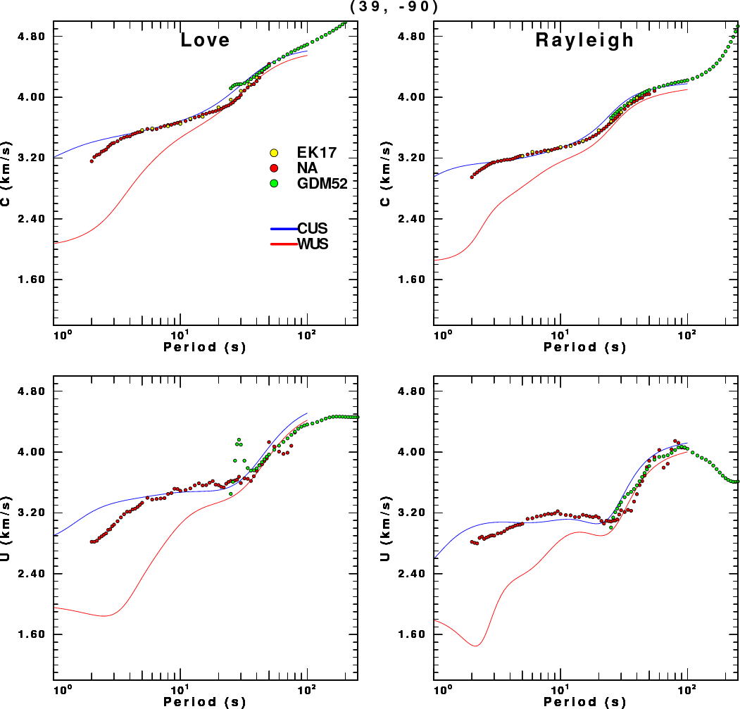
To evaluate the tomographic inversion, it was necessary to write shell scripts that would convert the tomography results to a format used by the Computer Programs in Seismology codes to eventually make a dispersion plot for a specific location. One such plot shown below was made for 39.0N and 90.0W.
The tomography currently consists of dispersion observations made from earthquake recordings and from inter-station Greens functions from noise-autocorrelation. The earthquake data are essential to obtain Love wave group velocities at periods greater than about 30 sec and often at the very short periods. The dispersion based on the noise-autocorrelation can provide better path coverage since one does not have to wait for an earthquake at the proper location.
In the current inversion, the dispersion from ground noise is weighted 4-times greater than the earthquake data to provide approximately equal numbers of observations.
Once the great-circle path tomography is performed, the results must be interpolated to estiamte the dispersion at a location. The tomography code and often at the very short periods. The dispersion based on the noise-autocorrelation can provide better path coverage since one does not have to wait for an earthquake at the proper location.
In the current inversion, the dispersion from ground noise is weighted 4-times greater than the earthquake data to provide approximately equal numbers of observations.
Once the great-circle path tomography is performed, the results must be interpolated to estiamte the dispersion at a location. The tomography code uses an approximate 100x100 km grid with a node at the center of each cell. The output provides the group velocity at a node and also a summation of all path segments through the corresponding cell. The codes distributed here, e.g., doquad.f estiamte the dispersion at a specified geographical coordinate by a two-dimensional interpolation. Since the tomography code default is to place the continental average at a node if there are no paths through the correspodning cell, this summation of all path segments is used to decide whether to use actuallyestimate a value. The present codes require the that path lengths be greater than 50 km for each of the nodes surrounding the specified position. If this is not true, no dispersion estiamte is returned. This is why gaps will appear or there is a limited range of periods for certain locations, e.g., 26N -98W,
Download the latest AMMON.CEUS.FINE.tgz Last Changed November 30, 2017
Unpack and tailor for your system with the following steps:
gunzip -c AMMON.CEUS.FINE.tgz | tar xf -
AMMON.CEUS.FINE/
               /00DISTRIBUTION.txt    - this file
               /Ekstrom17/            - the Ekstrom phase velocity from USArray
                         /EMKDSP      - shell script to make dispersion
                         /00README
                         /Lovec/      - files for Ekstorm Love phase velocity
                         /Rayleighc   - files for Ekstorm Rayleigh phase velocity
               /nGRIDREGION/FDODISP   - shell script to gets the dispersion from
                                        Ekstrom (2017), Ekstromglobal GDM52 and the SLU
                                        tomography. This also overlays theoretical dispersion
                                        for the CUS and WUS models if you have created
                                        the ${GREEDDIR}/Models, ${GREENDIR}/CUS.REG/SW and
                                        ${GREENDIR}/WUS.REG/SW.  GREENDIR is an environment parameter,
                                        that points to the location of the GREEN function directory.
                                        An example of setting this is the following line in
                                        my .bashrc:
                                              export GREENDIR='/d/rbh/GREEN'
               /GDM52/
                         /DOGDM52       A script to get values from GDM52
                         /GDM52_dispersion_sample1.out
                         /GDM52_dispersion.f
               [The following are the SLU tomography results for phase and group velocity for
                Love and Rayleigh waves. The FMKDSP script knows the mapping
                of period to the unique file number]
               /LOVEc/
                         /vc_000_001.xyz
                         /vc_000_002.xyz
                         ...
                         /per.uniq
               /RAYLc/
                         /vc_000_001.xyz
                         /vc_000_002.xyz
                         ...
                         /per.uniq
               /LOVEU/
                         /vc_000_001.xyz
                         /vc_000_002.xyz
                         ...
                         /per.uniq
               /RAYLU/
                         /vc_000_001.xyz
                         /vc_000_002.xyz
                         ...
                         /per.uniq
               /bin/
                         /FMKDSP       A script to get all results and to make a plot. Computer Programs
                                       in seismology is required
               /src/
                         /doquad.f     An interpolation program to give dispersion at a point from the tables.
                         /Makefile
         cd AMMON.CEUS.FINE
         cd src
         make doquad clean
If you the the code from the subdirectory nGRIDREGION, then no change is required. If you want to run this from other parts of the system, or to permit others to run this from their logins, change the following line to an absolute path:
TOMOTOP=..
to something line
TOMOTOP=/home/rbh/AMMON.CEUS.FINE
then anyone can issue a command like
/home/rbh/AMMON.CEUS.FINE/nGRIDREGION/FDODISP 39 -90
         LOVEc/vc_001_001.xyz is of the form

         26.112 -111.252 3.393 0.00
         26.112 -111.001 3.393 0.00
         ..........................
         39.153 -90.264 3.260 562.44
         39.153 -89.974 3.179 505.54
         ..........................
where the columns are geocentric latitude, geocentric longitude (which is also geodetic longitude), the
phase velocity in km/s and the last column is the sum of the lengths of all rays through the cell.
For this first two entries, there are not data for the cells, and thus the velocitues are not for the cell but
represent an average for the data set. These are not used. The current program doquad has the following line
set in the src/doquad.f: dl=50.0, which means that unless the value of the last column if greater than 50 km for the four cells surrounding the desired latitude/longitude, the dispersion will not be output.
the output of Ekstrom (2017) was reformatted into a three column tabular format, where the columns are geocentric latitude, geocentric longitude (which is also geodetic longitude), the phase velocity in km/s. A quadrilateral interpolation is performed, but there can be no test on the usefulness of the results. Results are obtained by the command doquad -3.
Consider the following command:
       cd AMMON.CEUS.FINE
       cd nGRIDREGION
       FDODISP 39 -90
After this the directory contents will be
         rbh@query ~/TEST $ ls -lt
         total 676
         -rw-rw-r-- 1 rbh rbh  16974 Dec  1 07:31 all.disp
         -rw-rw-r-- 1 rbh rbh  90320 Dec  1 07:31 all.png
         -rw-rw-r-- 1 rbh rbh 352901 Dec  1 07:31 all.eps
         -rw-rw-r-- 1 rbh rbh 117023 Dec  1 07:31 ALL.PLT
         -rw-rw-r-- 1 rbh rbh   9426 Dec  1 07:31 tomona.disp
         -rw-rw-r-- 1 rbh rbh    660 Dec  1 07:31 tomoek.disp
         -rw-rw-r-- 1 rbh rbh   6888 Dec  1 07:31 tomogdm52.disp
The dispersion files, e.g., all.disp, are in SURF96 format (see PROGRAMS.330/DOC/OVERVIEW.pdf/cps330o.pdf).
The file all.disp is a concatenation of the three data sets: tomona.disp for SLU tomogrpahy, tomoek.disp for Ekstrom (2017) and tomogdm52 for the Ekstrom global data set. the first five lines of these files are
         ==> tomoek.disp <==
         SURF96 L C X 0 05 3.5673 0.05
         SURF96 R C X 0 05 3.2243 0.05
         SURF96 L C X 0 06 3.5895 0.05
         SURF96 R C X 0 06 3.2818 0.05
         SURF96 L C X 0 08 3.6182 0.05

         ==> tomogdm52.disp <==
         SURF96 L C X 0      25.00     4.1175 0.05
         SURF96 L U X 0      25.00     3.4500 0.05
         SURF96 L C X 0      26.00     4.1457 0.05
         SURF96 L U X 0      26.00     3.6081 0.05
         SURF96 L C X 0      27.00     4.1631 0.05

         ==> tomona.disp <==
         SURF96 R U X 0 2.000000 2.8037 0.05
         SURF96 L U X 0 2.000000 2.8127 0.05
         SURF96 R C X 0 2.000000 2.9257 0.05
         SURF96 L C X 0 2.000000 3.1450 0.05
         SURF96 R U X 0 2.100000 2.8021 0.05
The last column is not used in these results and is a position holder for an error in the velocity value.
The all.disp file can be used in the inversion programs surf96 or joint96.
The other files are the graphics output of FDODISP. ALL.PLT is the plot in CALPLOT format, all.eps the EPS version, and all.png is the corresponding PNG file, which is shown below:
| >/td> |