
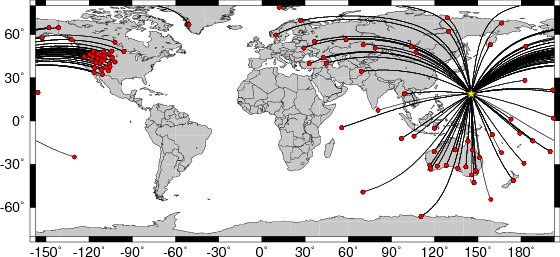
Location of the earthquake (yellow star) and great circle path from the epicenter to each station (red) [created using GMT (Wessel, P., and W. H. F. Smith, New version of Generic Mapping Tools released, EOS Trans. AGU, 76 329, 1995.)]
2007/10/31 03:30:19 18.84 145.32 240
The following compares this source inversion to the USGS Rapid Moment Tensor Solution and to the Harvard CMT solutions, if they are available.
 SLU Moment Tensor Solution
 2007/10/31 03:30:19

 Best Fitting Double Couple
    Mo = 8.81e+26 dyne-cm
    Mw = 7.23
    Z  = 210 km
     Plane   Strike  Dip  Rake
      NP1      196    64   134
      NP2      310    50    35
 Principal Axes:
   Axis    Value   Plunge  Azimuth
     T   8.81e+26     50     156
     N   0.00e+00     39     353
     P  -8.81e+26      8     256


 Moment Tensor: (dyne-cm)
    Component  Value
       Mxx     2.52e+26
       Mxy    -3.41e+26
       Mxz    -3.65e+26
       Myy    -7.50e+26
       Myz     2.99e+26
       Mzz     4.98e+26


                     ############--
                 #############---------
              ###############-------------
             #--------#####----------------
           ---------------##-----------------
          ---------------######---------------
         ---------------##########-------------
        ---------------#############------------
        ---------------###############----------
       ---------------#################----------
       --------------###################---------
       --------------#####################-------
       -   ----------#####################-------
         P ---------#######################-----
           ---------########################----
         -----------###########   ##########---
          ----------########### T ##########--
           ---------###########   ##########-
             -------#######################
              -------#####################
                 ----##################
                     -#############


 Harvard Convention
 Moment Tensor:
      R          T          F
  4.98e+26  -3.65e+26  -2.99e+26
 -3.65e+26   2.52e+26   3.41e+26
 -2.99e+26   3.41e+26  -7.50e+26
|
October 31, 2007, PAGAN REG., N. MARIANA ISLANDS, MW=7.2

Goran Ekstrom
Meredith Nettles

CENTROID-MOMENT-TENSOR  SOLUTION
GCMT EVENT:     C200710310330A
DATA: II IU CU IC GE
L.P.BODY WAVES:105S, 288C, T= 50
MANTLE WAVES:  103S, 263C, T=150
SURFACE WAVES: 107S, 274C, T= 50
TIMESTAMP:      Q-20071031122133
CENTROID LOCATION:
ORIGIN TIME:      03:30:26.0 0.1
LAT:18.87N 0.01;LON:145.60E 0.01
DEP:214.0  0.6;TRIANG HDUR:  9.9
MOMENT TENSOR: SCALE 10**27 D-CM
RR= 0.364 0.003; TT= 0.285 0.003
PP=-0.649 0.003; RT=-0.434 0.002
RP=-0.106 0.002; TP= 0.437 0.002
PRINCIPAL AXES:
1.(T) VAL=  0.857;PLG=42;AZM=160
2.(N)      -0.032;    48;    334
3.(P)      -0.825;     3;     67
BEST DBLE.COUPLE:M0= 8.41*10**26
NP1: STRIKE=195;DIP=59;SLIP= 150
NP2: STRIKE=302;DIP=64;SLIP=  35

            #########--
        ##########---------
      ###########------------
    ###########----------------
   --------###-----------------
  -----------###--------------- P
  ----------########-----------
 -----------###########-----------
 ----------##############---------
 ----------################-------
 ----------#################------
  --------####################---
  --------#########   #########--
   --------######## T #########-
    -------########   #########
      -----##################
        ----###############
            -##########
|
The following broadband stations passed the QC and were used for the source inversion. ADK AFI AGMN AHID ANMO ANTO ARU BBOO BILL BLDU BMO BOZ BRVK BW06 CAN CASY CHTO COCO COEN COLA COR CTAO DGMT DUG DZM EGAK EGMT EIDS ELK FFC FORT FUNA GNI HAWA HLID HNR HWUT ISCO KAPI KBL KBS KDAK KEV KIEV KIP KIV KMBL KONO KURK LAO LKWY MBWA MCQ MIDW MSEY MSO MVCO NEW NWAO OBN OGNE PAF PALK PET PFO POHA PTCN RAO RAR RLMT RSSD SDCO SFJD SNZO STKA TARA TAU TIXI TLY TOO TPNV TUC ULN WRAB WRAK WUAZ WVOR XMAS XMIS YAK YNG
All observed and Greens function waveforms are corrected to instrument response to ground velocity in meters/sec for the passband of 0.004 - 5 Hz. The traces were then lowpass filtered at 0.25 Hz and interpolated to a sample rate of 1 second.
For the grid search, the observed traces and Green's functions are read in an cut using the following commands
#####
#	Driver script for the teleseismic waveform inversion
#
#	The depth HS must be of the form 0010 for a depth of 1.0 km
#       of 6700 for a depth of 670.0 km
#
#	The Filter_Band is an integer with the following meansing
#
#	FILTER_BAND	1/FH	1/FL
#	1		60	12	for Mw < 6.4
#	2		100	20	6.4 =< Mw < 6.8
#	3		120	40	6.8 =< Mw < 7.2
#	4		143	80	7.2 =< Mw < 9.3
#####
#	Source duration - halfwidth of triangular function
#	this filters only the Green functions
#
#	halfwidth = 1.05 * 10-8 * M0^1/3 (M0 is dyne-cm)
#
#	MW	   half-width (sec)
#	5.0         0.75
#	6.0         2.45
#	7.0         7.7
#	8.0        24.5
#	9.0        74.3
#                       0.5*(MW - 9)
#  or half-width=74.3*10
#  or echo 7.23 |  awk '{print 74.3*exp(0.5*log(10.0)*(2100 - 9.0)) }'
#####
#  Processing window for P (use SAC variable A for P arrival
#  	Start   A  - 30
#  	End     A  + 2*HALFWIDTH + 0.03*HS + 30 + 1/FH
#  Processing window for SH (use SAC variable T0 for SH arrival
#  	Start   T0 - 60
#  	End     T0 + 2*HALFWIDTH + 0.06*HS + 30 + 1/FH
#  Processing window for SV (use SAC variable T1 for SV arrival
#  	Start   T1 - 60
#  	End     T1 + 2*HALFWIDTH + 0.06*HS + 30 + 1/FH
#
#	The term involving HS serves to include the depth phases and
#	to exclude the PP or SS at most distanace
#####
The cut windows attempt to include the P, pP, sP, pS, S and sS arrivals. However, oen must be very careful about the fact that PP may be included in some distance ranges.
The waveforms are then bandpass filtered by the application of the following high- and low-pass stages (an optional microseism filter):
hp c 0.0070 2
lp c 0.0125 2
int
br c 0.12 0.25 n 4 p 2
The traces were next integrated to ground displacment in meters. Finally the observed data are interpolated to ahve the same sampling at the Green's functions.
The source inversion is a multipass operation since a lower frequency filter band is used for larger earthquakes and since a search is made over depth. Up to three passed of the outer loop are made, after which the moment magnitude is determined and filter settings readjusted. The inner loop over depth samples all depths from 0 to 800 km with 5 km increments in depth to 50 km, followed by 10 km depth sampling for the remaining range.
The following filter ranges are used according to the moment magnitude Mw:
   FILTER_BAND   1/FH(s)  1/FL(s)
       1           60     12      Mw < 6.4
       2          100     20      6.4 < Mw <= 6.9
       3          120     40      Mw > 6.9
The map displays the distribution of stations used for this source inversion.
|
Location of the earthquake (yellow star) and great circle path from the epicenter to each station (red) [created using GMT (Wessel, P., and W. H. F. Smith, New version of Generic Mapping Tools released, EOS Trans. AGU, 76 329, 1995.)] |
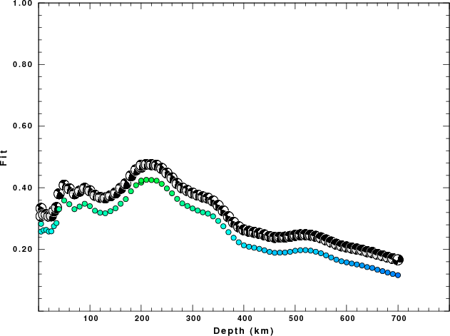
For this data set the favored solution is
WVFGRD96 210.0 310 50 35 7.23 0.4256
The following figures show the sensitivity of the goodness of fit parameter so source depth, the waveform comparison as a function of epicentral distance in degrees and the source to station azimuth
|
| Goodness of fit as a function of source depth. The measure is 1 - SUM (o -p)2 / SUM o2. A value of 1.0 is the best fit. The best double couple mechanism for the solution depth is plotted above goodness of fit value to indicate how the mefhanism may change with depth. |
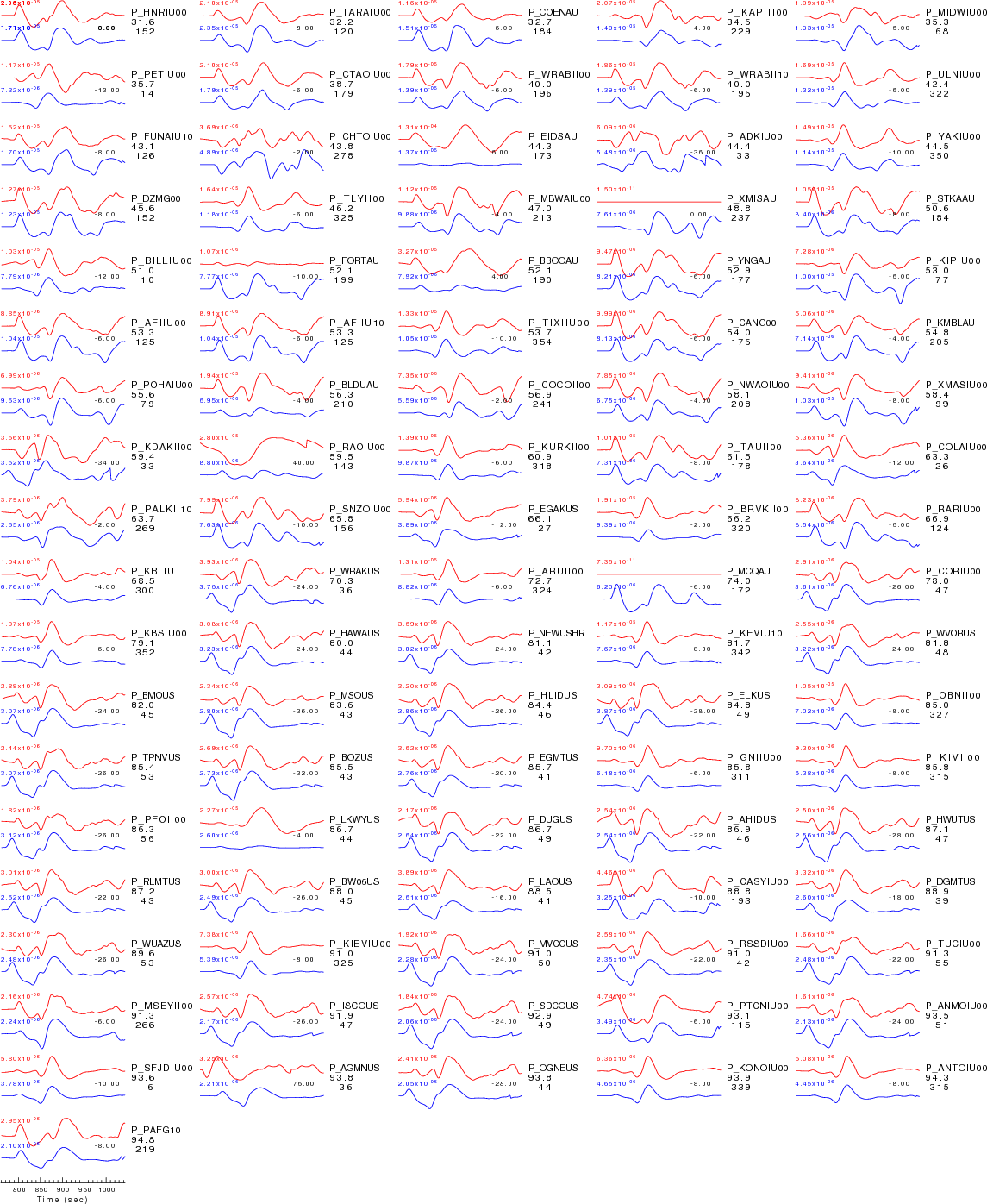
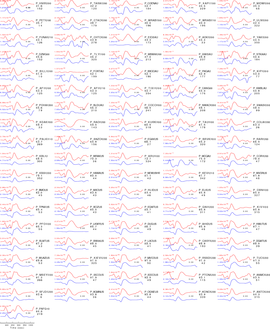
| P-wave Z component |
|
| Comparison of the observed traces (red) and solution predicted traces (blue) ordered in terms of increasing epicentral distance. Each pair of traces is annotated with the station name, epicentral distance in degrees, source to station azimuth in degrees. Each pair of traces is plotted with the same scale and the peak amplitudes are indicated at the lect of each trace. Finally the time shift between the P-wave first arrival picked and the the theoretical P-wave first arrival in the predicted trace is indicated, with a positive sign indicating that the predicted trace has been shifted to the right by the given number of seconds. as a function of source to station azimuth in degrees (D). The purpose of this display is to highlight the azimuthal dependence on the first motion. The traces are annotated with the station name at the top. |
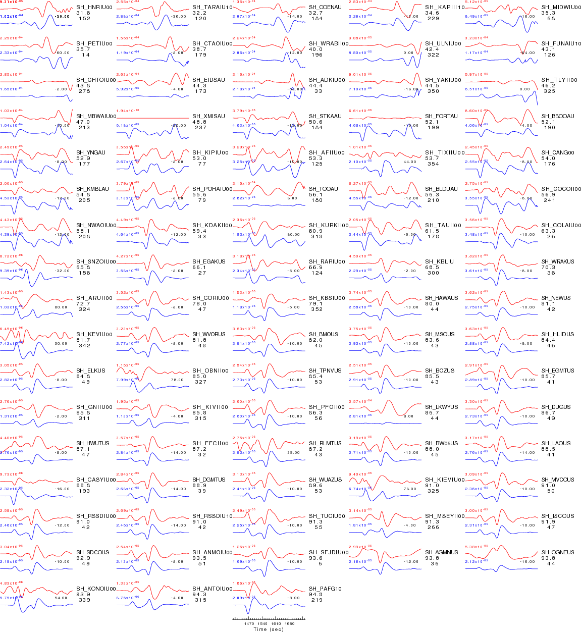
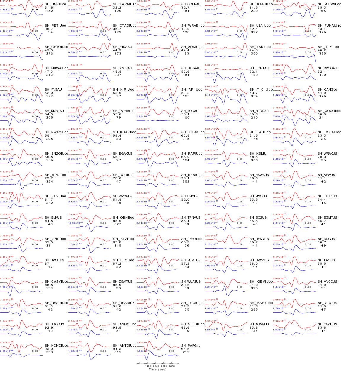
| SH-wave T component |
|
| Comparison of the observed traces (red) and solution predicted traces (blue) ordered in terms of increasing epicentral distance. Each pair of traces is annotated with the station name, epicentral distance in degrees, source to station azimuth in degrees. Each pair of traces is plotted with the same scale and the peak amplitudes are indicated at the lect of each trace. Finally the time shift between the P-wave first arrival picked and the the theoretical P-wave first arrival in the predicted trace is indicated, with a positive sign indicating that the predicted trace has been shifted to the right by the given number of seconds. as a function of source to station azimuth in degrees (D). The purpose of this display is to highlight the azimuthal dependence on the first motion. The traces are annotated with the station name at the top. |
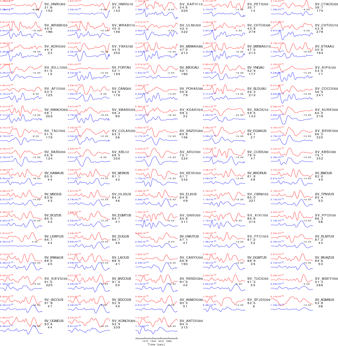
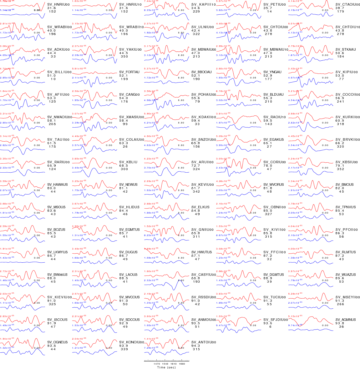
| SV-wave R component |
|
| Comparison of the observed traces (red) and solution predicted traces (blue) ordered in terms of increasing epicentral distance. Each pair of traces is annotated with the station name, epicentral distance in degrees, source to station azimuth in degrees. Each pair of traces is plotted with the same scale and the peak amplitudes are indicated at the lect of each trace. Finally the time shift between the P-wave first arrival picked and the the theoretical P-wave first arrival in the predicted trace is indicated, with a positive sign indicating that the predicted trace has been shifted to the right by the given number of seconds. as a function of source to station azimuth in degrees (D). The purpose of this display is to highlight the azimuthal dependence on the first motion. The traces are annotated with the station name at the top. |
All observed and Greens function waveforms are corrected to instrument response to ground velocity in meters/sec for the passband of 0.004 - 5 Hz. The traces were then lowpass filtered at 0.25 Hz and interpolated to a sample rate of 1 second.
The moment tensor solution used has the parameters:
HS=214
STK=195
DIP=59
RAKE=150
MW=7.2

The Green's function closest to the desired depth was
DEP=2100 , where (DEP/10) is the computed depth.
The cut windows attempt to include the P, pP, sP, pS, S and sS arrivals. However, one must be very careful about the fact that PP may be included in some distance ranges.
The waveforms are then bandpass filtered by the application of the following high- and low-pass stages (an optional microseism filter):
hp c 0.0070 2
lp c 0.0125 2
int
br c 0.12 0.25 n 4 p 2
The traces were next integrated to ground displacment in meters. Finally the observed data are interpolated to ahve the same sampling at the Green's functions.
The following filter ranges are used according to the moment magnitude Mw:
   FILTER_BAND   1/FH(s)  1/FL(s)
       1           60     12      Mw < 6.4
       2          100     20      6.4 < Mw <= 6.9
       3          120     40      Mw > 6.9
The map displays the distribution of stations used for this source inversion.
Location of the earthquake (yellow star) and great circle path from the epicenter to each station (red) [created using GMT (Wessel, P., and W. H. F. Smith, New version of Generic Mapping Tools released, EOS Trans. AGU, 76 329, 1995.)] |
| P-wave Z component |
|
| Comparison of the observed traces (red) and solution predicted traces (blue) ordered in terms of increasing epicentral distance. Each pair of traces is annotated with the station name, epicentral distance in degrees, source to station azimuth in degrees. Each pair of traces is plotted with the same scale and the peak amplitudes are indicated at the left of each trace. Finally the time shift between the P-wave first arrival picked and the the theoretical P-wave first arrival in the predicted trace is indicated, with a positive sign indicating that the predicted trace has been shifted to the right by the given number of seconds. as a function of source to station azimuth in degrees (D). The purpose of this display is to highlight the azimuthal dependence on the first motion. The traces are annotated with the station name at the top. |
| SH-wave T component |
|
| Comparison of the observed traces (red) and solution predicted traces (blue) ordered in terms of increasing epicentral distance. Each pair of traces is annotated with the station name, epicentral distance in degrees, source to station azimuth in degrees. Each pair of traces is plotted with the same scale and the peak amplitudes are indicated at the left of each trace. Finally the time shift between the P-wave first arrival picked and the the theoretical P-wave first arrival in the predicted trace is indicated, with a positive sign indicating that the predicted trace has been shifted to the right by the given number of seconds. as a function of source to station azimuth in degrees (D). The purpose of this display is to highlight the azimuthal dependence on the first motion. The traces are annotated with the station name at the top. |
| SV-wave R component |
|
| Comparison of the observed traces (red) and solution predicted traces (blue) ordered in terms of increasing epicentral distance. Each pair of traces is annotated with the station name, epicentral distance in degrees, source to station azimuth in degrees. Each pair of traces is plotted with the same scale and the peak amplitudes are indicated at the left of each trace. Finally the time shift between the P-wave first arrival picked and the the theoretical P-wave first arrival in the predicted trace is indicated, with a positive sign indicating that the predicted trace has been shifted to the right by the given number of seconds. as a function of source to station azimuth in degrees (D). The purpose of this display is to highlight the azimuthal dependence on the first motion. The traces are annotated with the station name at the top. |
Starting Processing         : Wed Nov 7 18:51:08 UTC 2007
Starting wget to get files  : Wed Nov 7 18:55:27 UTC 2007
Unpacking SEED volume       : Wed Nov 7 18:55:27 UTC 2007
Starting deconvolution      : Wed Nov 7 18:55:31 UTC 2007
Starting trace rotation     : Wed Nov 7 18:57:56 UTC 2007
Starting distance selection : Wed Nov 7 18:58:14 UTC 2007
Starting trace QC           : Wed Nov 7 18:58:22 UTC 2007
Starting Grid Search        : Wed Nov 7 19:04:19 UTC 2007
Starting documentation      : Wed Nov 7 20:13:54 UTC 2007
Processing Completion       : Wed Nov 7 20:13:55 UTC 2007