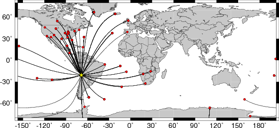
Location of the earthquake (yellow star) and great circle path from the epicenter to each station (red) [created using GMT (Wessel, P., and W. H. F. Smith, New version of Generic Mapping Tools released, EOS Trans. AGU, 76 329, 1995.)]
2007/10/25 08:35:17 -20.64 -68.46 101
The following compares this source inversion to the USGS Rapid Moment Tensor Solution and to the Harvard CMT solutions, if they are available.
The following broadband stations passed the QC and were used for the source inversion. ANMO ASCN BBSR BORG CASY CCM CMLA DWPF EFI ESK FFC HKT HOPE HRV JTS LSZ MCQ PAB PFO PMSA POHA PPBLO PPCWF PPMOO PPNAF PPNVW PPUHS PTCN RAR RCBR RPN RSSD SBA SFJD SHEL SJG SSPA SUR TEIG TRIS TSUM TUC WCI WVT XMAS
All observed and Greens function waveforms are corrected to instrument response to ground velocity in meters/sec for the passband of 0.004 - 5 Hz. The traces were then lowpass filtered at 0.25 Hz and interpolated to a sample rate of 1 second.
The moment tensor solution used has the parameters:
HS=122.2
STK=191
DIP=31
RAKE=-37
MW=5.6

The Green's function closest to the desired depth was
DEP=1200 , where (DEP/10) is the computed depth.
The cut windows attempt to include the P, pP, sP, pS, S and sS arrivals. However, one must be very careful about the fact that PP may be included in some distance ranges.
The waveforms are then bandpass filtered by the application of the following high- and low-pass stages (an optional microseism filter):
hp c 0.0167 2
lp c 0.0833 2
int
br c 0.12 0.25 n 4 p 2
The traces were next integrated to ground displacment in meters. Finally the observed data are interpolated to ahve the same sampling at the Green's functions.
The following filter ranges are used according to the moment magnitude Mw:
   FILTER_BAND   1/FH(s)  1/FL(s)
       1           60     12      Mw < 6.4
       2          100     20      6.4 < Mw <= 6.9
       3          120     40      Mw > 6.9
The map displays the distribution of stations used for this source inversion.
|
Location of the earthquake (yellow star) and great circle path from the epicenter to each station (red) [created using GMT (Wessel, P., and W. H. F. Smith, New version of Generic Mapping Tools released, EOS Trans. AGU, 76 329, 1995.)] |
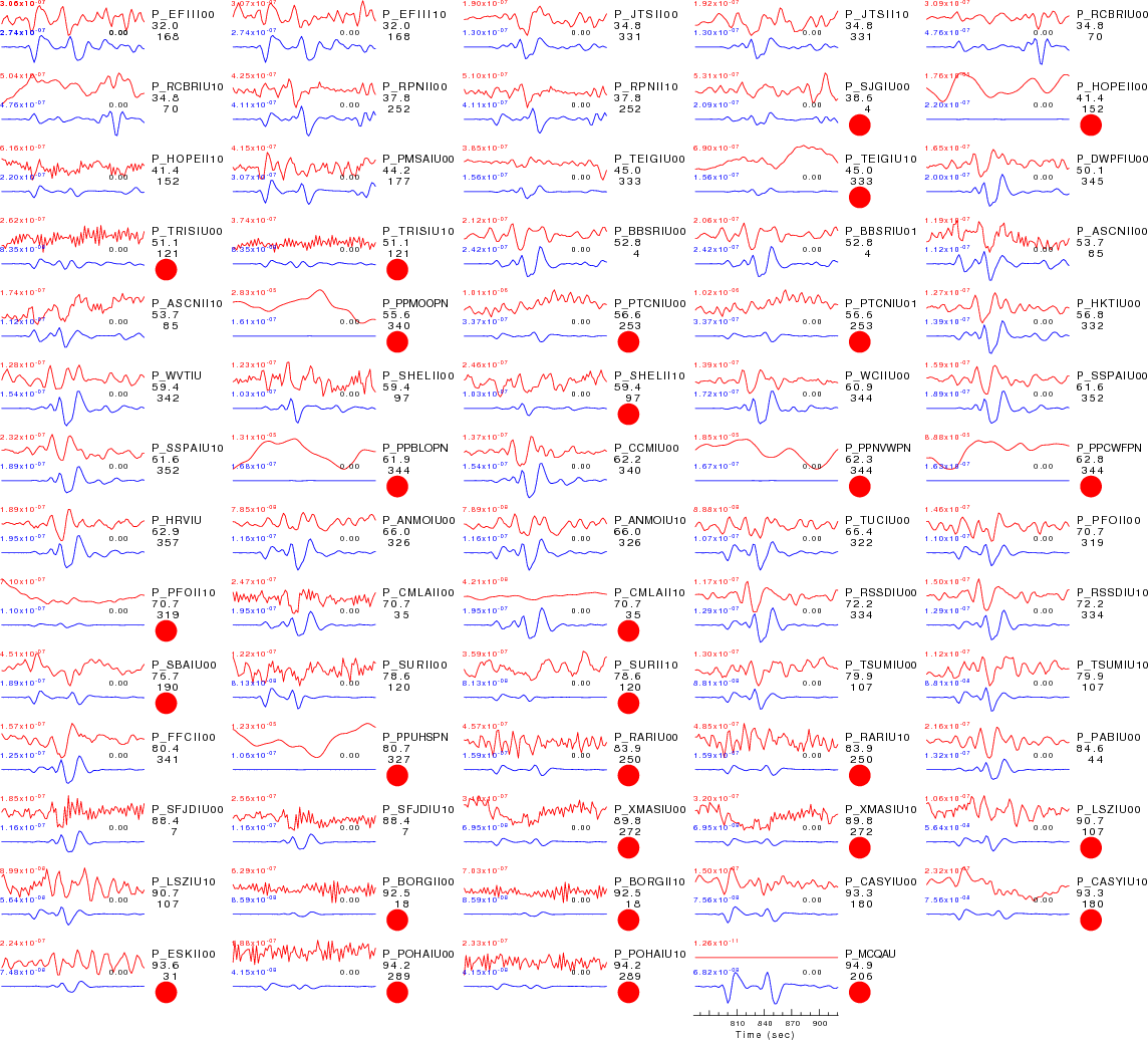
| P-wave Z component |
|
| Comparison of the observed traces (red) and solution predicted traces (blue) ordered in terms of increasing epicentral distance. Each pair of traces is annotated with the station name, epicentral distance in degrees, source to station azimuth in degrees. Each pair of traces is plotted with the same scale and the peak amplitudes are indicated at the left of each trace. Finally the time shift between the P-wave first arrival picked and the the theoretical P-wave first arrival in the predicted trace is indicated, with a positive sign indicating that the predicted trace has been shifted to the right by the given number of seconds. as a function of source to station azimuth in degrees (D). The purpose of this display is to highlight the azimuthal dependence on the first motion. The traces are annotated with the station name at the top. Trace units are in meters. |
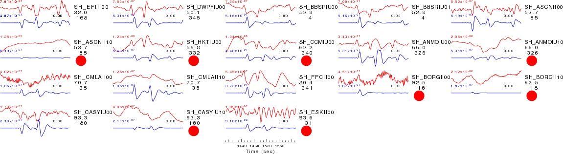
| SH-wave T component |
|
| Comparison of the observed traces (red) and solution predicted traces (blue) ordered in terms of increasing epicentral distance. Each pair of traces is annotated with the station name, epicentral distance in degrees, source to station azimuth in degrees. Each pair of traces is plotted with the same scale and the peak amplitudes are indicated at the left of each trace. Finally the time shift between the P-wave first arrival picked and the the theoretical P-wave first arrival in the predicted trace is indicated, with a positive sign indicating that the predicted trace has been shifted to the right by the given number of seconds. as a function of source to station azimuth in degrees (D). The purpose of this display is to highlight the azimuthal dependence on the first motion. The traces are annotated with the station name at the top. Trace units are in meters. |
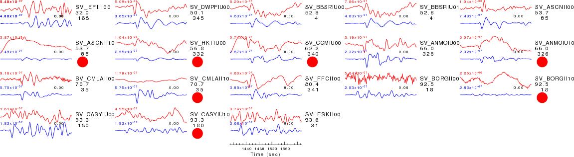
| SV-wave R component |
|
| Comparison of the observed traces (red) and solution predicted traces (blue) ordered in terms of increasing epicentral distance. Each pair of traces is annotated with the station name, epicentral distance in degrees, source to station azimuth in degrees. Each pair of traces is plotted with the same scale and the peak amplitudes are indicated at the left of each trace. Finally the time shift between the P-wave first arrival picked and the the theoretical P-wave first arrival in the predicted trace is indicated, with a positive sign indicating that the predicted trace has been shifted to the right by the given number of seconds. as a function of source to station azimuth in degrees (D). The purpose of this display is to highlight the azimuthal dependence on the first motion. The traces are annotated with the station name at the top. Trace units are in meters. |
Starting Processing         : Sat Nov 10 15:07:12 UTC 2007
Starting wget to get files  : Sat Nov 10 15:07:26 UTC 2007
Unpacking SEED volume       : Sat Nov 10 15:07:26 UTC 2007
Starting deconvolution      : Sat Nov 10 15:07:27 UTC 2007
Starting trace rotation     : Sat Nov 10 15:08:07 UTC 2007
Starting distance selection : Sat Nov 10 15:08:15 UTC 2007
Starting trace QC           : Sat Nov 10 15:08:18 UTC 2007
Starting synthetic          : Sat Nov 10 15:08:18 UTC 2007
Starting documentation      : Sat Nov 10 15:08:45 UTC 2007
Processing Completion       : Sat Nov 10 15:08:46 UTC 2007