
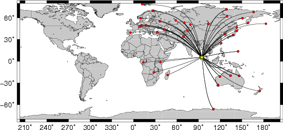
Location of the earthquake (yellow star) and great circle path from the epicenter to each station (red) [created using GMT (Wessel, P., and W. H. F. Smith, New version of Generic Mapping Tools released, EOS Trans. AGU, 76 329, 1995.)]
2007/04/27 08:02:48 5.35 94.61 30
The following compares this source inversion to the USGS Rapid Moment Tensor Solution and to the Harvard CMT solutions, if they are available.
 SLU Moment Tensor Solution
 2007/04/27 08:02:48

 Best Fitting Double Couple
    Mo = 5.69e+24 dyne-cm
    Mw = 5.77
    Z  = 35 km
     Plane   Strike  Dip  Rake
      NP1      130    70    85
      NP2      324    21   103
 Principal Axes:
   Axis    Value   Plunge  Azimuth
     T   5.69e+24     65      32
     N   0.00e+00      5     132
     P  -5.69e+24     25     224


 Moment Tensor: (dyne-cm)
    Component  Value
       Mxx    -1.68e+24
       Mxy    -1.87e+24
       Mxz     3.43e+24
       Myy    -1.96e+24
       Myz     2.66e+24
       Mzz     3.64e+24


                     --------------
                 -#############--------
              #####################-------
             #########################-----
           -############################-----
          ---############################-----
         -----################   ##########----
        -------############### T ###########----
        ---------#############   ###########----
       -----------###########################----
       -------------#########################----
       --------------#########################---
       ----------------#######################---
        ------------------####################--
        --------------------#################---
         ----------------------##############--
          ------   ---------------##########--
           ----- P -------------------######-
             ---   -----------------------#
              ---------------------------#
                 ----------------------
                     --------------


 Harvard Convention
 Moment Tensor:
      R          T          F
  3.64e+24   3.43e+24  -2.66e+24
  3.43e+24  -1.68e+24   1.87e+24
 -2.66e+24   1.87e+24  -1.96e+24
|
 07/04/27 08:02:48.79
 NORTHERN SUMATRA, INDONESIA
 Epicenter:   5.332   94.606
 MW 5.9

 USGS MOMENT TENSOR SOLUTION
 Depth  37         No. of sta: 38
 Moment Tensor;   Scale 10**17 Nm
   Mrr= 6.91       Mtt=-3.26
   Mpp=-3.64       Mrt= 5.40
   Mrp=-4.58       Mtp= 1.74
  Principal axes:
   T  Val= 10.18  Plg=65  Azm= 38
   N       -1.75       2      133
   P       -8.43      25      224

 Best Double Couple:Mo=9.3*10**17
  NP1:Strike=320 Dip=20 Slip=  97
  NP2:       132     70        87

               -------
          -----------------
        ###############------
      ####################-----
    ---#####################-----
   -----#####################-----
   ------###########   #######----
  --------########## T ########----
  ---------#########   #########---
  -----------###################---
  -------------##################--
  ---------------################--
   ----------------#############--
   -----   -----------##########--
    ---- P --------------######--
      --   -------------------#
        ---------------------
          -----------------
               -------
|
GS research CMT: maintained and developed by Jascha Polet at UC Santa Barbara.
This is a research system and solutions are *not* official USGS earthquake magnitudes.
AUTOMATIC solution, not reviewed by a seismologist
--------------------------------------------------
General region :  2007bran NORTHERN SUMATRA, INDONES
surface waves  (3.0,3.5,7,7.5 mHz)
Stations used :  AAK INCN KURK MAJO TLY ULN
Origin time: 2007  117   8   2  48
Original location (lat,lon,depth) :      5.30000    94.6000  30
Moment tensor (x1.e26 dyncm) :
Mrr :      0.101869 Mtt :     -0.027792
Mff :     -0.074076 Mrt :      0.039980
Mrf :     -0.006005 Mtf :      0.040412
T-axis:  moment=     0.113   plunge=    73.631  azimuth=   353.953
N-axis:  moment=    -0.013   plunge=    14.480  azimuth=   145.498
P-axis:  moment=    -0.101   plunge=     7.471  azimuth=   237.439
best double couple: Mo=    0.107(x1.e26 dyncm)  Mw=6.0  tau=  2.6
nodal planes (strike/dip/slip):  343.68/ 39.61/113.09     134.72/ 54.09/ 72.02
Centroid location :    4.115    94.098    55.583
Centroid time :     -8.953
Variance reduction (%) :  21

                   ***********
               ****-oooooo--- ****
            ***----------oooo--   ***
          **----------------ooo-     **
         **o------------------oo--    **
        *--o-------------------oo--     *
       * --o--------------------oo-      *
      **  -oo--------------------oo-     **
      *    -o-----------T---------oo-     *
     **     oo---------------------o-     **
     **      oo---------+----------o-     **
     **       ooo------------------oo     **
      *         oo------------------o     *
      **         ooo---------------oo    **
       *           ooo-------------o     *
        *P           oooo---------oo    *
         **             ooooo-----o   **
          **                ooooooooo**
            ***                ooo***
               ****          o****
                   ***********

          0-   30-  60-  90-  120- 150- 180- 210- 240- 270- 300- 330-
z-comp:     0    0    0    0    2    1    2    0    0    0    0    0
r-comp:     0    0    0    0    1    2    0    0    0    0    0    0
t-comp:     0    0    0    0    1    2    1    0    0    0    0    0
Total number of traces used =  12
number of runs = 9
starttime = Fri Apr 27 02:22:29 MDT 2007
endtime = Fri Apr 27 02:40:59 MDT 2007
inversion time = Fri Apr 27 02:40:57 MDT 2007 - Fri Apr 27 02:40:59 MDT 2007
Solution produced by inversion of channels with var red > 2%
|
The following broadband stations passed the QC and were used for the source inversion. AAK ABPO ADK ANTO ARU BFO BILL BRVK CASY CTAO ERM GRFO GUMO INCN KBL KBS KEV KIV KMBO KONO KURK LSZ MA2 MAJO MBWA MORC MSKU NWAO OBN PAB PET SNZO TATO TIXI TLY WRAB YAK YSS
All observed and Greens function waveforms are corrected to instrument response to ground velocity in meters/sec for the passband of 0.004 - 5 Hz. The traces were then lowpass filtered at 0.25 Hz and interpolated to a sample rate of 1 second.
For the deviatoric moment tensor inversion, the observed traces and Green's functions are read in an cut using the following commands
#####
#	Driver script for the teleseismic waveform inversion
#
#	The depth HS must be of the form 0010 for a depth of 1.0 km
#       of 6700 for a depth of 670.0 km
#
#	The Filter_Band is an integer with the following meansing
#
#	FILTER_BAND	1/FH	1/FL
#	1		60	12	for Mw < 6.4
#	2		100	20	6.4 =< Mw < 6.8
#	3		120	40	6.8 =< Mw < 7.2
#	4		143	80	7.2 =< Mw < 9.3
#####
#	Source duration - halfwidth of triangular function
#	this filters only the Green functions
#
#	halfwidth = 1.05 * 10-8 * M0^1/3 (M0 is dyne-cm)
#
#	MW	   half-width (sec)
#	5.0         0.75
#	6.0         2.45
#	7.0         7.7
#	8.0        24.5
#	9.0        74.3
#                       0.5*(MW - 9)
#  or half-width=74.3*10
#  or echo 5.82 |  awk '{print 74.3*exp(0.5*log(10.0)*(0300 - 9.0)) }'
#####
#  Processing window for P (use SAC variable A for P arrival
#  	Start   A  - 30
#  	End     A  + 2*HALFWIDTH + 0.03*HS + 30 + 1/FH
#  Processing window for SH (use SAC variable T0 for SH arrival
#  	Start   T0 - 60
#  	End     T0 + 2*HALFWIDTH + 0.06*HS + 30 + 1/FH
#  Processing window for SV (use SAC variable T1 for SV arrival
#  	Start   T1 - 60
#  	End     T1 + 2*HALFWIDTH + 0.06*HS + 30 + 1/FH
#
#	The term involving HS serves to include the depth phases and
#	to exclude the PP or SS at most distanace
#####
The cut windows attempt to include the P, pP, sP, pS, S and sS arrivals. However, oen must be very careful about the fact that PP may be included in some distance ranges.
The waveforms are then bandpass filtered by the application of the following high- and low-pass stages (an optional microseism filter):
hp c 0.0167 2
lp c 0.0833 2
int
br c 0.12 0.25 n 4 p 2
The traces were next integrated to ground displacment in meters. Finally the observed data are interpolated to ahve the same sampling at the Green's functions.
The source inversion is a multipass operation since a lower frequency filter band is used for larger earthquakes and since a search is made over depth. Up to three passed of the outer loop are made, after which the moment magnitude is determined and filter settings readjusted. The inner loop over depth samples all depths from 0 to 800 km with 5 km increments in depth to 50 km, followed by 10 km depth sampling for the remaining range.
The following filter ranges are used according to the moment magnitude Mw:
   FILTER_BAND   1/FH(s)  1/FL(s)
       1           60     12      Mw < 6.4
       2          100     20      6.4 < Mw <= 6.9
       3          120     40      Mw > 6.9
The map displays the distribution of stations used for this source inversion.
|
Location of the earthquake (yellow star) and great circle path from the epicenter to each station (red) [created using GMT (Wessel, P., and W. H. F. Smith, New version of Generic Mapping Tools released, EOS Trans. AGU, 76 329, 1995.)] |
For this data set the favored solution is
WVFMTD96 30.0 128. 62. 90. 5.82 0.575 0.412E-06 0.569 0.758 0.200E-06 56.7
The following figures show the sensitivity of the goodness of fit parameter so source depth, the waveform comparison as a function of epicentral distance in degrees and the source to station azimuth
|
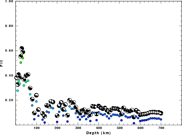
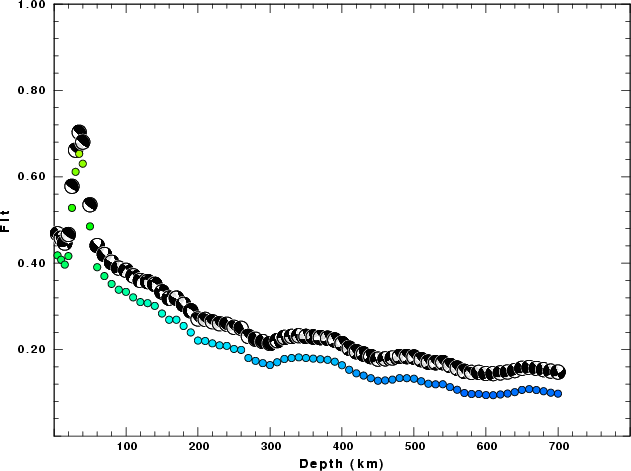
| Goodness of fit as a function of source depth. The measure is 1 - SUM (o -p)2 / SUM o2. A value of 1.0 is the best fit. The best double couple mechanism for the solution depth is plotted above goodness of fit value to indicate how the mefhanism may change with depth. |
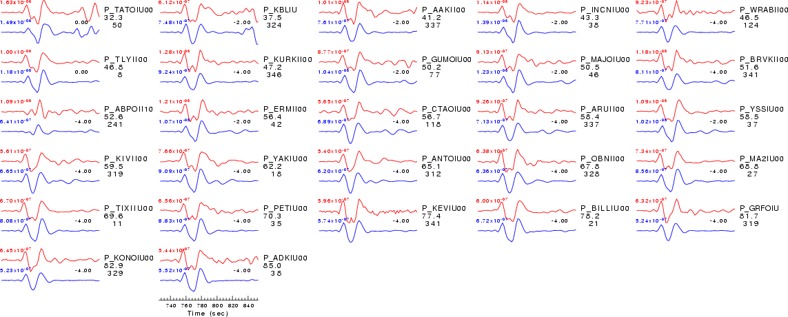
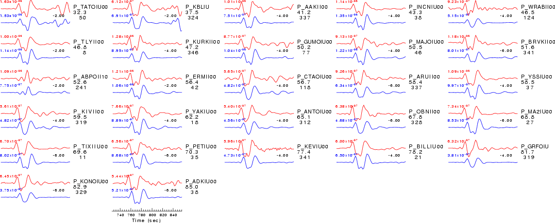
| P-wave Z component |
|
| Comparison of the observed traces (red) and solution predicted traces (blue) ordered in terms of increasing epicentral distance. Each pair of traces is annotated with the station name, epicentral distance in degrees, source to station azimuth in degrees. Each pair of traces is plotted with the same scale and the peak amplitudes are indicated at the lect of each trace. Finally the time shift between the P-wave first arrival picked and the the theoretical P-wave first arrival in the predicted trace is indicated, with a positive sign indicating that the predicted trace has been shifted to the right by the given number of seconds. as a function of source to station azimuth in degrees (D). The purpose of this display is to highlight the azimuthal dependence on the first motion. The traces are annotated with the station name at the top. |
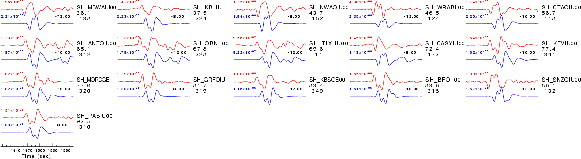
| SH-wave T component |
|
| Comparison of the observed traces (red) and solution predicted traces (blue) ordered in terms of increasing epicentral distance. Each pair of traces is annotated with the station name, epicentral distance in degrees, source to station azimuth in degrees. Each pair of traces is plotted with the same scale and the peak amplitudes are indicated at the lect of each trace. Finally the time shift between the P-wave first arrival picked and the the theoretical P-wave first arrival in the predicted trace is indicated, with a positive sign indicating that the predicted trace has been shifted to the right by the given number of seconds. as a function of source to station azimuth in degrees (D). The purpose of this display is to highlight the azimuthal dependence on the first motion. The traces are annotated with the station name at the top. |
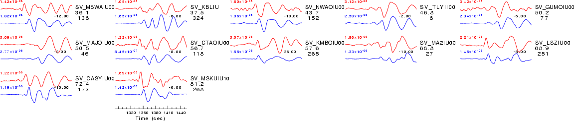
| SV-wave R component |
|
| Comparison of the observed traces (red) and solution predicted traces (blue) ordered in terms of increasing epicentral distance. Each pair of traces is annotated with the station name, epicentral distance in degrees, source to station azimuth in degrees. Each pair of traces is plotted with the same scale and the peak amplitudes are indicated at the lect of each trace. Finally the time shift between the P-wave first arrival picked and the the theoretical P-wave first arrival in the predicted trace is indicated, with a positive sign indicating that the predicted trace has been shifted to the right by the given number of seconds. as a function of source to station azimuth in degrees (D). The purpose of this display is to highlight the azimuthal dependence on the first motion. The traces are annotated with the station name at the top. |
All observed and Greens function waveforms are corrected to instrument response to ground velocity in meters/sec for the passband of 0.004 - 5 Hz. The traces were then lowpass filtered at 0.25 Hz and interpolated to a sample rate of 1 second.
For the grid search, the observed traces and Green's functions are read in an cut using the following commands
#####
#	Driver script for the teleseismic waveform inversion
#
#	The depth HS must be of the form 0010 for a depth of 1.0 km
#       of 6700 for a depth of 670.0 km
#
#	The Filter_Band is an integer with the following meansing
#
#	FILTER_BAND	1/FH	1/FL
#	1		60	12	for Mw < 6.4
#	2		100	20	6.4 =< Mw < 6.8
#	3		120	40	6.8 =< Mw < 7.2
#	4		143	80	7.2 =< Mw < 9.3
#####
#	Source duration - halfwidth of triangular function
#	this filters only the Green functions
#
#	halfwidth = 1.05 * 10-8 * M0^1/3 (M0 is dyne-cm)
#
#	MW	   half-width (sec)
#	5.0         0.75
#	6.0         2.45
#	7.0         7.7
#	8.0        24.5
#	9.0        74.3
#                       0.5*(MW - 9)
#  or half-width=74.3*10
#  or echo 5.77 |  awk '{print 74.3*exp(0.5*log(10.0)*(0350 - 9.0)) }'
#####
#  Processing window for P (use SAC variable A for P arrival
#  	Start   A  - 30
#  	End     A  + 2*HALFWIDTH + 0.03*HS + 30 + 1/FH
#  Processing window for SH (use SAC variable T0 for SH arrival
#  	Start   T0 - 60
#  	End     T0 + 2*HALFWIDTH + 0.06*HS + 30 + 1/FH
#  Processing window for SV (use SAC variable T1 for SV arrival
#  	Start   T1 - 60
#  	End     T1 + 2*HALFWIDTH + 0.06*HS + 30 + 1/FH
#
#	The term involving HS serves to include the depth phases and
#	to exclude the PP or SS at most distanace
#####
The cut windows attempt to include the P, pP, sP, pS, S and sS arrivals. However, oen must be very careful about the fact that PP may be included in some distance ranges.
The waveforms are then bandpass filtered by the application of the following high- and low-pass stages (an optional microseism filter):
hp c 0.0167 2
lp c 0.0833 2
int
br c 0.12 0.25 n 4 p 2
The traces were next integrated to ground displacment in meters. Finally the observed data are interpolated to ahve the same sampling at the Green's functions.
The source inversion is a multipass operation since a lower frequency filter band is used for larger earthquakes and since a search is made over depth. Up to three passed of the outer loop are made, after which the moment magnitude is determined and filter settings readjusted. The inner loop over depth samples all depths from 0 to 800 km with 5 km increments in depth to 50 km, followed by 10 km depth sampling for the remaining range.
The following filter ranges are used according to the moment magnitude Mw:
   FILTER_BAND   1/FH(s)  1/FL(s)
       1           60     12      Mw < 6.4
       2          100     20      6.4 < Mw <= 6.9
       3          120     40      Mw > 6.9
The map displays the distribution of stations used for this source inversion.
Location of the earthquake (yellow star) and great circle path from the epicenter to each station (red) [created using GMT (Wessel, P., and W. H. F. Smith, New version of Generic Mapping Tools released, EOS Trans. AGU, 76 329, 1995.)] |
For this data set the favored solution is
WVFGRD96 35.0 130 70 85 5.77 0.6532
The following figures show the sensitivity of the goodness of fit parameter so source depth, the waveform comparison as a function of epicentral distance in degrees and the source to station azimuth
|
| Goodness of fit as a function of source depth. The measure is 1 - SUM (o -p)2 / SUM o2. A value of 1.0 is the best fit. The best double couple mechanism for the solution depth is plotted above goodness of fit value to indicate how the mefhanism may change with depth. |
| P-wave Z component |
|
| Comparison of the observed traces (red) and solution predicted traces (blue) ordered in terms of increasing epicentral distance. Each pair of traces is annotated with the station name, epicentral distance in degrees, source to station azimuth in degrees. Each pair of traces is plotted with the same scale and the peak amplitudes are indicated at the lect of each trace. Finally the time shift between the P-wave first arrival picked and the the theoretical P-wave first arrival in the predicted trace is indicated, with a positive sign indicating that the predicted trace has been shifted to the right by the given number of seconds. as a function of source to station azimuth in degrees (D). The purpose of this display is to highlight the azimuthal dependence on the first motion. The traces are annotated with the station name at the top. |
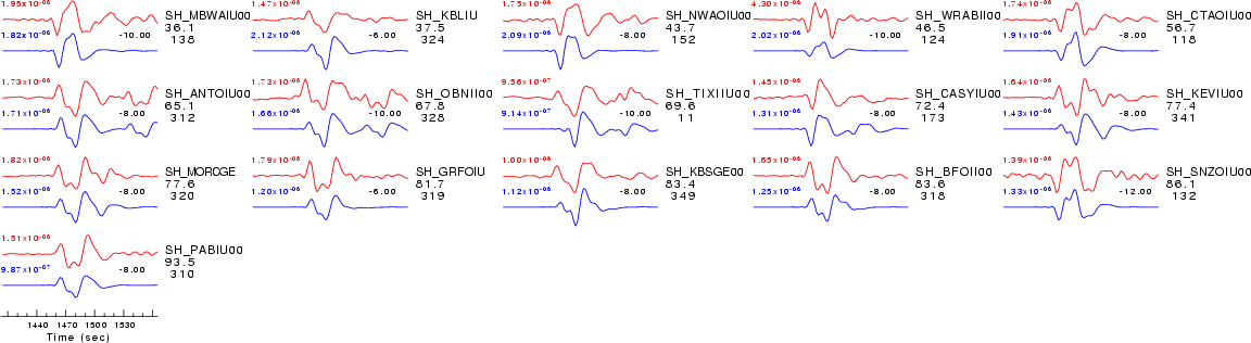
| SH-wave T component |
|
| Comparison of the observed traces (red) and solution predicted traces (blue) ordered in terms of increasing epicentral distance. Each pair of traces is annotated with the station name, epicentral distance in degrees, source to station azimuth in degrees. Each pair of traces is plotted with the same scale and the peak amplitudes are indicated at the lect of each trace. Finally the time shift between the P-wave first arrival picked and the the theoretical P-wave first arrival in the predicted trace is indicated, with a positive sign indicating that the predicted trace has been shifted to the right by the given number of seconds. as a function of source to station azimuth in degrees (D). The purpose of this display is to highlight the azimuthal dependence on the first motion. The traces are annotated with the station name at the top. |
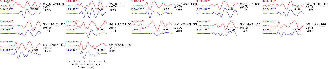
| SV-wave R component |
|
| Comparison of the observed traces (red) and solution predicted traces (blue) ordered in terms of increasing epicentral distance. Each pair of traces is annotated with the station name, epicentral distance in degrees, source to station azimuth in degrees. Each pair of traces is plotted with the same scale and the peak amplitudes are indicated at the lect of each trace. Finally the time shift between the P-wave first arrival picked and the the theoretical P-wave first arrival in the predicted trace is indicated, with a positive sign indicating that the predicted trace has been shifted to the right by the given number of seconds. as a function of source to station azimuth in degrees (D). The purpose of this display is to highlight the azimuthal dependence on the first motion. The traces are annotated with the station name at the top. |
Starting Processing         : Fri Apr 27 15:15:00 UTC 2007
Starting query to get files : Fri Apr 27 15:15:00 UTC 2007
Starting stareq for response: Fri Apr 27 15:20:58 UTC 2007
Starting deconvolution      : Fri Apr 27 15:23:34 UTC 2007
Starting trace rotation     : Fri Apr 27 15:24:53 UTC 2007
Starting distance selection : Fri Apr 27 15:25:13 UTC 2007
Starting trace QC           : Fri Apr 27 15:25:20 UTC 2007
Starting Grid Search        : Fri Apr 27 15:28:37 UTC 2007
Starting MTD                : Fri Apr 27 15:37:40 UTC 2007
Starting documentation      : Fri Apr 27 15:43:02 UTC 2007