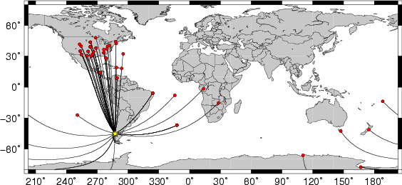
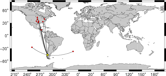
Location of the earthquake (yellow star) and great circle path from the epicenter to each station (red) [created using GMT (Wessel, P., and W. H. F. Smith, New version of Generic Mapping Tools released, EOS Trans. AGU, 76 329, 1995.)]
2007/04/21 17:53:47 -45.27 -72.49 38
The following compares this source inversion to the USGS Rapid Moment Tensor Solution and to the Harvard CMT solutions, if they are available.
 SLU Moment Tensor Solution
 2007/04/21 17:53:47

 Best Fitting Double Couple
    Mo = 1.97e+25 dyne-cm
    Mw = 6.13
    Z  = 5 km
     Plane   Strike  Dip  Rake
      NP1      196    64   -146
      NP2       90    60   -30
 Principal Axes:
   Axis    Value   Plunge  Azimuth
     T   1.97e+25      3     322
     N   0.00e+00     49     229
     P  -1.97e+25     41      55


 Moment Tensor: (dyne-cm)
    Component  Value
       Mxx     8.54e+24
       Mxy    -1.48e+25
       Mxz    -4.93e+24
       Myy     3.60e+17
       Myz    -8.54e+24
       Mzz    -8.54e+24


                     ############--
                 ##############--------
               T ############-------------
             #   ##########----------------
           ###############-------------------
          ###############---------------------
         ###############------------   --------
        ###############------------- P ---------
        ###############-------------   ---------
       ###############---------------------------
       ##############----------------------------
       -#############---------------------------#
       ---###########-------------------------###
        ------######----------------------######
        -----------#-----------------###########
         -----------###########################
          ----------##########################
           ---------#########################
             -------#######################
              -------#####################
                 ----##################
                     -#############


 Harvard Convention
 Moment Tensor:
      R          T          F
 -8.54e+24  -4.93e+24   8.54e+24
 -4.93e+24   8.54e+24   1.48e+25
  8.54e+24   1.48e+25   3.60e+17
|
07/04/21 17:53:47.12
 AISEN, CHILE
 Epicenter: -45.266  -72.496
 MW 6.2

 USGS MOMENT TENSOR SOLUTION
 Depth  13         No. of sta:  9
 Moment Tensor;   Scale 10**18 Nm
   Mrr=-0.25       Mtt= 0.40
   Mpp=-0.15       Mrt=-0.02
   Mrp= 0.13       Mtp= 2.48
  Principal axes:
   T  Val=  2.62  Plg= 1  Azm=318
   N       -0.25      87      203
   P       -2.37       3       48

 Best Double Couple:Mo=2.5*10**18
  NP1:Strike= 93 Dip=87 Slip=  -1
  NP2:       183     89      -177

               ####---
          #########--------
       T ##########----------
         ##########---------- P
    ###############----------   -
   ################---------------
   ################---------------
  #################----------------
  ################-----------------
  --------########-----------------
  ----------------#################
  ----------------#################
   ---------------################
   ---------------################
    --------------###############
      ------------#############
        ----------###########
          --------#########
               ---####
|
April 21, 2007, AISEN, CHILE, MW=6.2

Goran Ekstrom
Meredith Nettles

CENTROID-MOMENT-TENSOR  SOLUTION
GCMT EVENT:     C200704211753A
DATA: II IU CU IC
L.P.BODY WAVES: 89S, 179C, T= 40
MANTLE WAVES:   82S, 148C, T=125
SURFACE WAVES:  77S, 169C, T= 50
TIMESTAMP:      Q-20070421211730
CENTROID LOCATION:
ORIGIN TIME:      17:53:48.5 0.1
LAT:45.39S 0.01;LON: 72.89W 0.01
DEP: 12.0  FIX;TRIANG HDUR:  3.2
MOMENT TENSOR: SCALE 10**25 D-CM
RR=-0.798 0.018; TT=-0.232 0.019
PP= 1.030 0.021; RT= 0.493 0.049
RP= 0.170 0.050; TP= 2.680 0.016
PRINCIPAL AXES:
1.(T) VAL=  3.201;PLG= 6;AZM=309
2.(N)      -0.796;    78;     70
3.(P)      -2.405;    10;    218
BEST DBLE.COUPLE:M0= 2.80*10**25
NP1: STRIKE=353;DIP=78;SLIP=-177
NP2: STRIKE=263;DIP=87;SLIP= -12

            ####-------
        #########----------
       ##########------------
     T ###########-------------
   #   ###########--------------
  #################--------------
  #################--------------
 ###################--------------
 ###################-#############
 ######-------------##############
 -------------------##############
  ------------------#############
  ------------------#############
   -----------------############
    ---   ----------###########
      - P ----------#########
          ----------#######
            --------###
|
USGS research CMT: maintained and developed by Jascha Polet at UC Santa Barbara.
This is a research system and solutions are *not* official USGS earthquake magnitudes.
AUTOMATIC solution, not reviewed by a seismologist
--------------------------------------------------
General region :  2007bkba AISEN, CHILE
surface waves  (3.0,3.5,7,7.5 mHz)
Stations used : CASY NNA PMSA RPN SDV SJG SUR
Origin time: 2007  111  17  53  47
Original location (lat,lon,depth) :     -45.3000   -72.5000  38
Moment tensor (x1.e26 dyncm) :
Mrr :     -0.171273 Mtt :     -0.006392
Mff :      0.177665 Mrt :      0.042590
Mrf :      0.197695 Mtf :      0.238976
T-axis:  moment=     0.404   plunge=    18.313  azimuth=   301.933
N-axis:  moment=    -0.123   plunge=    31.036  azimuth=   200.445
P-axis:  moment=    -0.281   plunge=    52.859  azimuth=    57.844
best double couple: Mo=    0.342(x1.e26 dyncm)  Mw=6.3  tau=  3.9
nodal planes (strike/dip/slip):   70.32/ 38.20/-33.52     187.82/ 70.03/-123.27
Centroid location :  -45.220   -72.729    28.942
Centroid time :     -5.391
Variance reduction (%) :  18

                   ***********
               ****-----ooo   ****
            ***--------oo         ***
          **-----------o             **
         **-----------oo              **
        *------------oo                 *
       *---T---------o                   *
      **------------oo                   **
      *-------------o          P         o*
     **-------------o                   oo**
     **------------oo   +               o **
     **------------o                  oo -**
      *----------- o                 oo---*
      **--------   o               ooo---**
       *oo----     o             ooo-----*
        *oooo      o         ooooo------*
         ** oooooooo  oooooooo   -----**
          **       oooo        ------**
            ***     o         ----***
               **** oo      --****
                   ***********

          0-   30-  60-  90-  120- 150- 180- 210- 240- 270- 300- 330-
z-comp:     1    0    1    0    0    2    0    0    1    0    0    1
r-comp:     1    0    0    0    0    1    1    0    1    0    0    1
t-comp:     1    0    0    0    0    1    1    0    1    0    0    1
Total number of traces used =  16
number of runs = 12
starttime = Sat Apr 21 12:15:42 MDT 2007
endtime = Sat Apr 21 12:43:29 MDT 2007
inversion time = Sat Apr 21 12:43:22 MDT 2007 - Sat Apr 21 12:43:29 MDT 2007
Solution produced by inversion of all available channels
|
The following broadband stations passed the QC and were used for the source inversion. AFI ANMO ASCN BBSR BLA CASY CCM DWPF ECSD EYMN GOGA HKT HRV ISCO JCT KSU1 LBNH LSZ MCWV MIAR MNTX MSKU NATX RCBR RPN RWWY SBA SDDR SDV SJG SNZO SSPA TAU TGUH TRIS TZTN WMOK
All observed and Greens function waveforms are corrected to instrument response to ground velocity in meters/sec for the passband of 0.004 - 5 Hz. The traces were then lowpass filtered at 0.25 Hz and interpolated to a sample rate of 1 second.
For the deviatoric moment tensor inversion, the observed traces and Green's functions are read in an cut using the following commands
#####
#	Driver script for the teleseismic waveform inversion
#
#	The depth HS must be of the form 0010 for a depth of 1.0 km
#       of 6700 for a depth of 670.0 km
#
#	The Filter_Band is an integer with the following meansing
#
#	FILTER_BAND	1/FH	1/FL
#	1		60	12	for Mw < 6.4
#	2		100	20	6.4 =< Mw < 6.8
#	3		120	40	6.8 =< Mw < 7.2
#	4		143	80	7.2 =< Mw < 9.3
#####
#	Source duration - halfwidth of triangular function
#	this filters only the Green functions
#
#	halfwidth = 1.05 * 10-8 * M0^1/3 (M0 is dyne-cm)
#
#	MW	   half-width (sec)
#	5.0         0.75
#	6.0         2.45
#	7.0         7.7
#	8.0        24.5
#	9.0        74.3
#                       0.5*(MW - 9)
#  or half-width=74.3*10
#  or echo 6.25 |  awk '{print 74.3*exp(0.5*log(10.0)*(0700 - 9.0)) }'
#####
#  Processing window for P (use SAC variable A for P arrival
#  	Start   A  - 30
#  	End     A  + 2*HALFWIDTH + 0.03*HS + 30 + 1/FH
#  Processing window for SH (use SAC variable T0 for SH arrival
#  	Start   T0 - 60
#  	End     T0 + 2*HALFWIDTH + 0.06*HS + 30 + 1/FH
#  Processing window for SV (use SAC variable T1 for SV arrival
#  	Start   T1 - 60
#  	End     T1 + 2*HALFWIDTH + 0.06*HS + 30 + 1/FH
#
#	The term involving HS serves to include the depth phases and
#	to exclude the PP or SS at most distanace
#####
The cut windows attempt to include the P, pP, sP, pS, S and sS arrivals. However, oen must be very careful about the fact that PP may be included in some distance ranges.
The waveforms are then bandpass filtered by the application of the following high- and low-pass stages (an optional microseism filter):
hp c 0.0167 2
lp c 0.0833 2
int
br c 0.12 0.25 n 4 p 2
The traces were next integrated to ground displacment in meters. Finally the observed data are interpolated to ahve the same sampling at the Green's functions.
The source inversion is a multipass operation since a lower frequency filter band is used for larger earthquakes and since a search is made over depth. Up to three passed of the outer loop are made, after which the moment magnitude is determined and filter settings readjusted. The inner loop over depth samples all depths from 0 to 800 km with 5 km increments in depth to 50 km, followed by 10 km depth sampling for the remaining range.
The following filter ranges are used according to the moment magnitude Mw:
   FILTER_BAND   1/FH(s)  1/FL(s)
       1           60     12      Mw < 6.4
       2          100     20      6.4 < Mw <= 6.9
       3          120     40      Mw > 6.9
The map displays the distribution of stations used for this source inversion.
|
Location of the earthquake (yellow star) and great circle path from the epicenter to each station (red) [created using GMT (Wessel, P., and W. H. F. Smith, New version of Generic Mapping Tools released, EOS Trans. AGU, 76 329, 1995.)] |
For this data set the favored solution is
WVFMTD96 70.0 179. 77. -156. 6.26 0.316 0.138E-05 0.343 0.564 0.607E-06 24.4
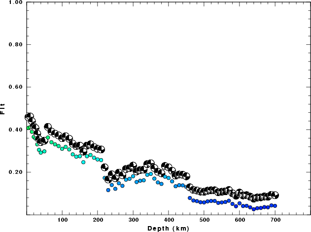
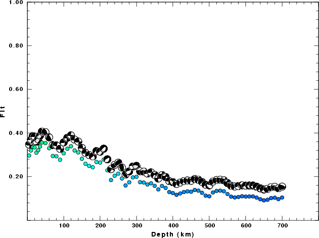
The following figures show the sensitivity of the goodness of fit parameter so source depth, the waveform comparison as a function of epicentral distance in degrees and the source to station azimuth
|
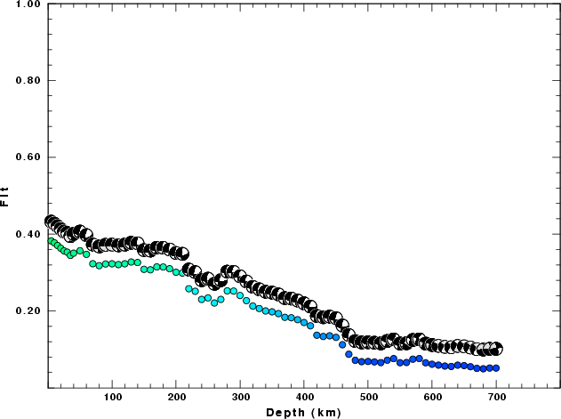
| Goodness of fit as a function of source depth. The measure is 1 - SUM (o -p)2 / SUM o2. A value of 1.0 is the best fit. The best double couple mechanism for the solution depth is plotted above goodness of fit value to indicate how the mefhanism may change with depth. |
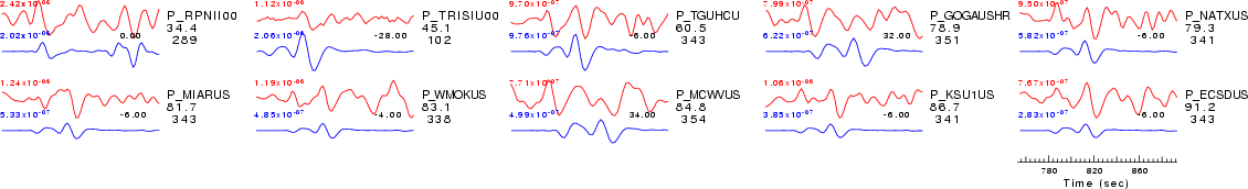
| P-wave Z component |
|
| Comparison of the observed traces (red) and solution predicted traces (blue) ordered in terms of increasing epicentral distance. Each pair of traces is annotated with the station name, epicentral distance in degrees, source to station azimuth in degrees. Each pair of traces is plotted with the same scale and the peak amplitudes are indicated at the lect of each trace. Finally the time shift between the P-wave first arrival picked and the the theoretical P-wave first arrival in the predicted trace is indicated, with a positive sign indicating that the predicted trace has been shifted to the right by the given number of seconds. as a function of source to station azimuth in degrees (D). The purpose of this display is to highlight the azimuthal dependence on the first motion. The traces are annotated with the station name at the top. |
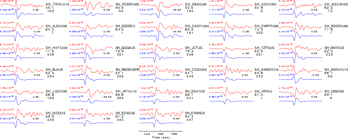
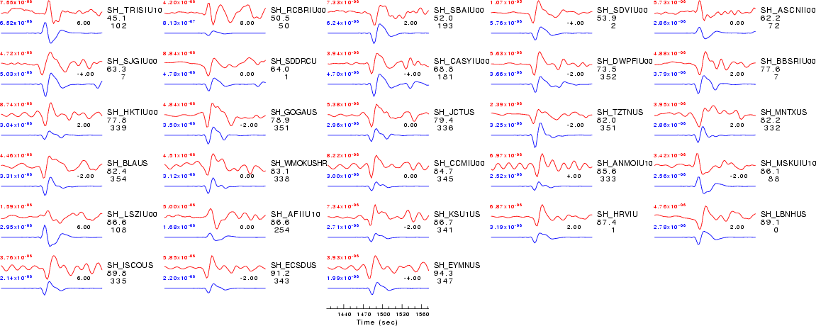
| SH-wave T component |
|
| Comparison of the observed traces (red) and solution predicted traces (blue) ordered in terms of increasing epicentral distance. Each pair of traces is annotated with the station name, epicentral distance in degrees, source to station azimuth in degrees. Each pair of traces is plotted with the same scale and the peak amplitudes are indicated at the lect of each trace. Finally the time shift between the P-wave first arrival picked and the the theoretical P-wave first arrival in the predicted trace is indicated, with a positive sign indicating that the predicted trace has been shifted to the right by the given number of seconds. as a function of source to station azimuth in degrees (D). The purpose of this display is to highlight the azimuthal dependence on the first motion. The traces are annotated with the station name at the top. |
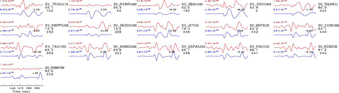
| SV-wave R component |
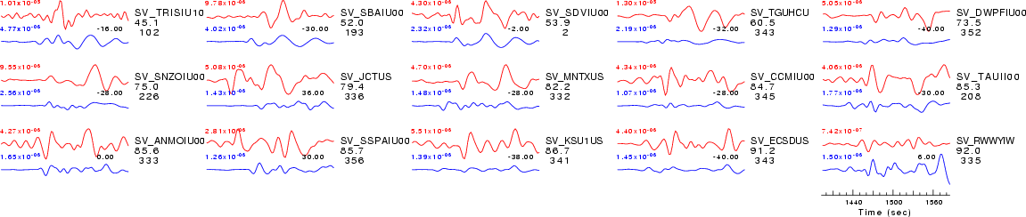
|
| Comparison of the observed traces (red) and solution predicted traces (blue) ordered in terms of increasing epicentral distance. Each pair of traces is annotated with the station name, epicentral distance in degrees, source to station azimuth in degrees. Each pair of traces is plotted with the same scale and the peak amplitudes are indicated at the lect of each trace. Finally the time shift between the P-wave first arrival picked and the the theoretical P-wave first arrival in the predicted trace is indicated, with a positive sign indicating that the predicted trace has been shifted to the right by the given number of seconds. as a function of source to station azimuth in degrees (D). The purpose of this display is to highlight the azimuthal dependence on the first motion. The traces are annotated with the station name at the top. |
All observed and Greens function waveforms are corrected to instrument response to ground velocity in meters/sec for the passband of 0.004 - 5 Hz. The traces were then lowpass filtered at 0.25 Hz and interpolated to a sample rate of 1 second.
For the deviatoric moment tensor inversion, the observed traces and Green's functions are read in an cut using the following commands
#####
#	Driver script for the teleseismic waveform inversion
#
#	The depth HS must be of the form 0010 for a depth of 1.0 km
#       of 6700 for a depth of 670.0 km
#
#	The Filter_Band is an integer with the following meansing
#
#	FILTER_BAND	1/FH	1/FL
#	1		60	12	for Mw < 6.4
#	2		100	20	6.4 =< Mw < 6.8
#	3		120	40	6.8 =< Mw < 7.2
#	4		143	80	7.2 =< Mw < 9.3
#####
#	Source duration - halfwidth of triangular function
#	this filters only the Green functions
#
#	halfwidth = 1.05 * 10-8 * M0^1/3 (M0 is dyne-cm)
#
#	MW	   half-width (sec)
#	5.0         0.75
#	6.0         2.45
#	7.0         7.7
#	8.0        24.5
#	9.0        74.3
#                       0.5*(MW - 9)
#  or half-width=74.3*10
#  or echo 6.41 |  awk '{print 74.3*exp(0.5*log(10.0)*(1200 - 9.0)) }'
#####
#  Processing window for P (use SAC variable A for P arrival
#  	Start   A  - 30
#  	End     A  + 2*HALFWIDTH + 0.03*HS + 30 + 1/FH
#  Processing window for SH (use SAC variable T0 for SH arrival
#  	Start   T0 - 60
#  	End     T0 + 2*HALFWIDTH + 0.06*HS + 30 + 1/FH
#  Processing window for SV (use SAC variable T1 for SV arrival
#  	Start   T1 - 60
#  	End     T1 + 2*HALFWIDTH + 0.06*HS + 30 + 1/FH
#
#	The term involving HS serves to include the depth phases and
#	to exclude the PP or SS at most distanace
#####
The cut windows attempt to include the P, pP, sP, pS, S and sS arrivals. However, oen must be very careful about the fact that PP may be included in some distance ranges.
The waveforms are then bandpass filtered by the application of the following high- and low-pass stages (an optional microseism filter):
hp c 0.0100 2
lp c 0.0500 2
int
br c 0.12 0.25 n 4 p 2
The traces were next integrated to ground displacment in meters. Finally the observed data are interpolated to ahve the same sampling at the Green's functions.
The source inversion is a multipass operation since a lower frequency filter band is used for larger earthquakes and since a search is made over depth. Up to three passed of the outer loop are made, after which the moment magnitude is determined and filter settings readjusted. The inner loop over depth samples all depths from 0 to 800 km with 5 km increments in depth to 50 km, followed by 10 km depth sampling for the remaining range.
The following filter ranges are used according to the moment magnitude Mw:
   FILTER_BAND   1/FH(s)  1/FL(s)
       1           60     12      Mw < 6.4
       2          100     20      6.4 < Mw <= 6.9
       3          120     40      Mw > 6.9
The map displays the distribution of stations used for this source inversion.

Location of the earthquake (yellow star) and great circle path from the epicenter to each station (red) [created using GMT (Wessel, P., and W. H. F. Smith, New version of Generic Mapping Tools released, EOS Trans. AGU, 76 329, 1995.)] |
For this data set the favored solution is
WVFMTD96 120.0 268. 88. -5. 6.41 0.144 0.488E-06 0.122 0.410 0.241E-06 67.4
The following figures show the sensitivity of the goodness of fit parameter so source depth, the waveform comparison as a function of epicentral distance in degrees and the source to station azimuth
|
|
| Goodness of fit as a function of source depth. The measure is 1 - SUM (o -p)2 / SUM o2. A value of 1.0 is the best fit. The best double couple mechanism for the solution depth is plotted above goodness of fit value to indicate how the mefhanism may change with depth. |
| P-wave Z component |
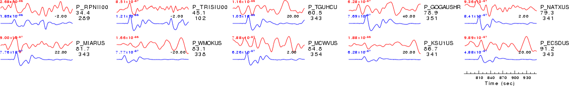
|
| Comparison of the observed traces (red) and solution predicted traces (blue) ordered in terms of increasing epicentral distance. Each pair of traces is annotated with the station name, epicentral distance in degrees, source to station azimuth in degrees. Each pair of traces is plotted with the same scale and the peak amplitudes are indicated at the lect of each trace. Finally the time shift between the P-wave first arrival picked and the the theoretical P-wave first arrival in the predicted trace is indicated, with a positive sign indicating that the predicted trace has been shifted to the right by the given number of seconds. as a function of source to station azimuth in degrees (D). The purpose of this display is to highlight the azimuthal dependence on the first motion. The traces are annotated with the station name at the top. |
All observed and Greens function waveforms are corrected to instrument response to ground velocity in meters/sec for the passband of 0.004 - 5 Hz. The traces were then lowpass filtered at 0.25 Hz and interpolated to a sample rate of 1 second.
For the grid search, the observed traces and Green's functions are read in an cut using the following commands
#####
#	Driver script for the teleseismic waveform inversion
#
#	The depth HS must be of the form 0010 for a depth of 1.0 km
#       of 6700 for a depth of 670.0 km
#
#	The Filter_Band is an integer with the following meansing
#
#	FILTER_BAND	1/FH	1/FL
#	1		60	12	for Mw < 6.4
#	2		100	20	6.4 =< Mw < 6.8
#	3		120	40	6.8 =< Mw < 7.2
#	4		143	80	7.2 =< Mw < 9.3
#####
#	Source duration - halfwidth of triangular function
#	this filters only the Green functions
#
#	halfwidth = 1.05 * 10-8 * M0^1/3 (M0 is dyne-cm)
#
#	MW	   half-width (sec)
#	5.0         0.75
#	6.0         2.45
#	7.0         7.7
#	8.0        24.5
#	9.0        74.3
#                       0.5*(MW - 9)
#  or half-width=74.3*10
#  or echo 6.12 |  awk '{print 74.3*exp(0.5*log(10.0)*(0050 - 9.0)) }'
#####
#  Processing window for P (use SAC variable A for P arrival
#  	Start   A  - 30
#  	End     A  + 2*HALFWIDTH + 0.03*HS + 30 + 1/FH
#  Processing window for SH (use SAC variable T0 for SH arrival
#  	Start   T0 - 60
#  	End     T0 + 2*HALFWIDTH + 0.06*HS + 30 + 1/FH
#  Processing window for SV (use SAC variable T1 for SV arrival
#  	Start   T1 - 60
#  	End     T1 + 2*HALFWIDTH + 0.06*HS + 30 + 1/FH
#
#	The term involving HS serves to include the depth phases and
#	to exclude the PP or SS at most distanace
#####
The cut windows attempt to include the P, pP, sP, pS, S and sS arrivals. However, oen must be very careful about the fact that PP may be included in some distance ranges.
The waveforms are then bandpass filtered by the application of the following high- and low-pass stages (an optional microseism filter):
hp c 0.0167 2
lp c 0.0833 2
int
br c 0.12 0.25 n 4 p 2
The traces were next integrated to ground displacment in meters. Finally the observed data are interpolated to ahve the same sampling at the Green's functions.
The source inversion is a multipass operation since a lower frequency filter band is used for larger earthquakes and since a search is made over depth. Up to three passed of the outer loop are made, after which the moment magnitude is determined and filter settings readjusted. The inner loop over depth samples all depths from 0 to 800 km with 5 km increments in depth to 50 km, followed by 10 km depth sampling for the remaining range.
The following filter ranges are used according to the moment magnitude Mw:
   FILTER_BAND   1/FH(s)  1/FL(s)
       1           60     12      Mw < 6.4
       2          100     20      6.4 < Mw <= 6.9
       3          120     40      Mw > 6.9
The map displays the distribution of stations used for this source inversion.

Location of the earthquake (yellow star) and great circle path from the epicenter to each station (red) [created using GMT (Wessel, P., and W. H. F. Smith, New version of Generic Mapping Tools released, EOS Trans. AGU, 76 329, 1995.)] |
For this data set the favored solution is
WVFGRD96 5.0 90 60 -30 6.13 0.3803
The following figures show the sensitivity of the goodness of fit parameter so source depth, the waveform comparison as a function of epicentral distance in degrees and the source to station azimuth
|
| Goodness of fit as a function of source depth. The measure is 1 - SUM (o -p)2 / SUM o2. A value of 1.0 is the best fit. The best double couple mechanism for the solution depth is plotted above goodness of fit value to indicate how the mefhanism may change with depth. |
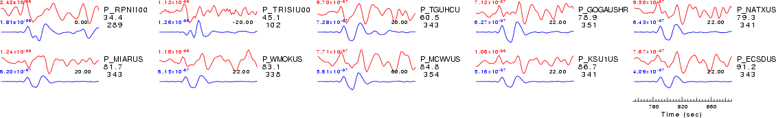
| P-wave Z component |
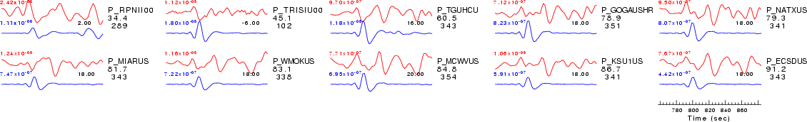
|
| Comparison of the observed traces (red) and solution predicted traces (blue) ordered in terms of increasing epicentral distance. Each pair of traces is annotated with the station name, epicentral distance in degrees, source to station azimuth in degrees. Each pair of traces is plotted with the same scale and the peak amplitudes are indicated at the lect of each trace. Finally the time shift between the P-wave first arrival picked and the the theoretical P-wave first arrival in the predicted trace is indicated, with a positive sign indicating that the predicted trace has been shifted to the right by the given number of seconds. as a function of source to station azimuth in degrees (D). The purpose of this display is to highlight the azimuthal dependence on the first motion. The traces are annotated with the station name at the top. |
| SH-wave T component |
|
| Comparison of the observed traces (red) and solution predicted traces (blue) ordered in terms of increasing epicentral distance. Each pair of traces is annotated with the station name, epicentral distance in degrees, source to station azimuth in degrees. Each pair of traces is plotted with the same scale and the peak amplitudes are indicated at the lect of each trace. Finally the time shift between the P-wave first arrival picked and the the theoretical P-wave first arrival in the predicted trace is indicated, with a positive sign indicating that the predicted trace has been shifted to the right by the given number of seconds. as a function of source to station azimuth in degrees (D). The purpose of this display is to highlight the azimuthal dependence on the first motion. The traces are annotated with the station name at the top. |
| SV-wave R component |
|
| Comparison of the observed traces (red) and solution predicted traces (blue) ordered in terms of increasing epicentral distance. Each pair of traces is annotated with the station name, epicentral distance in degrees, source to station azimuth in degrees. Each pair of traces is plotted with the same scale and the peak amplitudes are indicated at the lect of each trace. Finally the time shift between the P-wave first arrival picked and the the theoretical P-wave first arrival in the predicted trace is indicated, with a positive sign indicating that the predicted trace has been shifted to the right by the given number of seconds. as a function of source to station azimuth in degrees (D). The purpose of this display is to highlight the azimuthal dependence on the first motion. The traces are annotated with the station name at the top. |
All observed and Greens function waveforms are corrected to instrument response to ground velocity in meters/sec for the passband of 0.004 - 5 Hz. The traces were then lowpass filtered at 0.25 Hz and interpolated to a sample rate of 1 second.
For the grid search, the observed traces and Green's functions are read in an cut using the following commands
#####
#	Driver script for the teleseismic waveform inversion
#
#	The depth HS must be of the form 0010 for a depth of 1.0 km
#       of 6700 for a depth of 670.0 km
#
#	The Filter_Band is an integer with the following meansing
#
#	FILTER_BAND	1/FH	1/FL
#	1		60	12	for Mw < 6.4
#	2		100	20	6.4 =< Mw < 6.8
#	3		120	40	6.8 =< Mw < 7.2
#	4		143	80	7.2 =< Mw < 9.3
#####
#	Source duration - halfwidth of triangular function
#	this filters only the Green functions
#
#	halfwidth = 1.05 * 10-8 * M0^1/3 (M0 is dyne-cm)
#
#	MW	   half-width (sec)
#	5.0         0.75
#	6.0         2.45
#	7.0         7.7
#	8.0        24.5
#	9.0        74.3
#                       0.5*(MW - 9)
#  or half-width=74.3*10
#  or echo 6.10 |  awk '{print 74.3*exp(0.5*log(10.0)*(0400 - 9.0)) }'
#####
#  Processing window for P (use SAC variable A for P arrival
#  	Start   A  - 30
#  	End     A  + 2*HALFWIDTH + 0.03*HS + 30 + 1/FH
#  Processing window for SH (use SAC variable T0 for SH arrival
#  	Start   T0 - 60
#  	End     T0 + 2*HALFWIDTH + 0.06*HS + 30 + 1/FH
#  Processing window for SV (use SAC variable T1 for SV arrival
#  	Start   T1 - 60
#  	End     T1 + 2*HALFWIDTH + 0.06*HS + 30 + 1/FH
#
#	The term involving HS serves to include the depth phases and
#	to exclude the PP or SS at most distanace
#####
The cut windows attempt to include the P, pP, sP, pS, S and sS arrivals. However, oen must be very careful about the fact that PP may be included in some distance ranges.
The waveforms are then bandpass filtered by the application of the following high- and low-pass stages (an optional microseism filter):
hp c 0.0167 2
lp c 0.0833 2
int
br c 0.12 0.25 n 4 p 2
The traces were next integrated to ground displacment in meters. Finally the observed data are interpolated to ahve the same sampling at the Green's functions.
The source inversion is a multipass operation since a lower frequency filter band is used for larger earthquakes and since a search is made over depth. Up to three passed of the outer loop are made, after which the moment magnitude is determined and filter settings readjusted. The inner loop over depth samples all depths from 0 to 800 km with 5 km increments in depth to 50 km, followed by 10 km depth sampling for the remaining range.
The following filter ranges are used according to the moment magnitude Mw:
   FILTER_BAND   1/FH(s)  1/FL(s)
       1           60     12      Mw < 6.4
       2          100     20      6.4 < Mw <= 6.9
       3          120     40      Mw > 6.9
The map displays the distribution of stations used for this source inversion.
Location of the earthquake (yellow star) and great circle path from the epicenter to each station (red) [created using GMT (Wessel, P., and W. H. F. Smith, New version of Generic Mapping Tools released, EOS Trans. AGU, 76 329, 1995.)] |
For this data set the favored solution is
WVFGRD96 40.0 120 30 60 6.10 0.3570
The following figures show the sensitivity of the goodness of fit parameter so source depth, the waveform comparison as a function of epicentral distance in degrees and the source to station azimuth
|
| Goodness of fit as a function of source depth. The measure is 1 - SUM (o -p)2 / SUM o2. A value of 1.0 is the best fit. The best double couple mechanism for the solution depth is plotted above goodness of fit value to indicate how the mefhanism may change with depth. |
| P-wave Z component |
|
| Comparison of the observed traces (red) and solution predicted traces (blue) ordered in terms of increasing epicentral distance. Each pair of traces is annotated with the station name, epicentral distance in degrees, source to station azimuth in degrees. Each pair of traces is plotted with the same scale and the peak amplitudes are indicated at the lect of each trace. Finally the time shift between the P-wave first arrival picked and the the theoretical P-wave first arrival in the predicted trace is indicated, with a positive sign indicating that the predicted trace has been shifted to the right by the given number of seconds. as a function of source to station azimuth in degrees (D). The purpose of this display is to highlight the azimuthal dependence on the first motion. The traces are annotated with the station name at the top. |
Starting Processing         : Sat Apr 21 18:27:30 UTC 2007
Starting query to get files : Sat Apr 21 18:27:30 UTC 2007
Starting stareq for response: Sat Apr 21 18:36:28 UTC 2007
Starting deconvolution      : Sat Apr 21 18:38:30 UTC 2007
Starting trace rotation     : Sat Apr 21 18:40:28 UTC 2007
Starting distance selection : Sat Apr 21 18:41:12 UTC 2007
Starting trace QC           : Sat Apr 21 18:41:25 UTC 2007
Starting Grid Search        : Sat Apr 21 18:47:17 UTC 2007
Starting MTD                : Sat Apr 21 18:54:52 UTC 2007
Starting documentation      : Sat Apr 21 18:59:17 UTC 2007
Processing Completion       : Sat Apr 21 18:59:17 UTC 2007