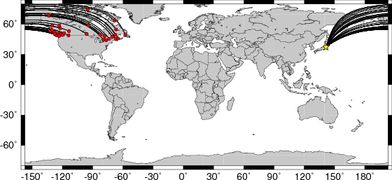
Location of the earthquake (yellow star) and great circle path from the epicenter to each station (red) [created using GMT (Wessel, P., and W. H. F. Smith, New version of Generic Mapping Tools released, EOS Trans. AGU, 76 329, 1995.)]
2007/11/26 13:51:39 37.40 141.57 39
The following compares this source inversion to the USGS Rapid Moment Tensor Solution and to the Harvard CMT solutions, if they are available.
The following broadband stations passed the QC and were used for the source inversion. BBB BMBC CBB DLBC DRLN EDB EDM FCC FNBB FRB GAC GGN HNB HOPB ICQ INK KAPO KGNO LLLB LMN LMQ MNT MOBC NLLB OZB PGC PHC PNT RES RUBB SADO SCHQ SHB SLEB SNB ULM VGZ VLDQ WALA
All observed and Greens function waveforms are corrected to instrument response to ground velocity in meters/sec for the passband of 0.004 - 5 Hz. The traces were then lowpass filtered at 0.25 Hz and interpolated to a sample rate of 1 second.
The moment tensor solution used has the parameters:
HS=40
STK=212
DIP=24
RAKE=100
MW=5.9

The Green's function closest to the desired depth was
DEP=0400 , where (DEP/10) is the computed depth.
The cut windows attempt to include the P, pP, sP, pS, S and sS arrivals. However, one must be very careful about the fact that PP may be included in some distance ranges.
The waveforms are then bandpass filtered by the application of the following high- and low-pass stages (an optional microseism filter):
hp c 0.0167 2
lp c 0.0833 2
int
br c 0.12 0.25 n 4 p 2
The traces were next integrated to ground displacment in meters. Finally the observed data are interpolated to have the same sampling at the Green's functions.
The following filter ranges are used according to the moment magnitude Mw:
   FILTER_BAND   1/FH(s)  1/FL(s)
       1           60     12      Mw < 6.4
       2          100     20      6.4 < Mw <= 6.9
       3          120     40      Mw > 6.9
The map displays the distribution of stations used for this source inversion.
|
Location of the earthquake (yellow star) and great circle path from the epicenter to each station (red) [created using GMT (Wessel, P., and W. H. F. Smith, New version of Generic Mapping Tools released, EOS Trans. AGU, 76 329, 1995.)] |
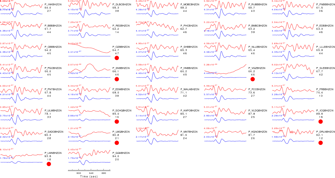
| P-wave Z component |
|
| Observed (red) and predicted seismograms (blue) ordered by increasing epicentral distance. Each pair of traces is annotated with the wave type and a station identifier (station, network, and channel id's), epicentral distance in degrees, source-to-station azimuth in degrees. Each seismogram pair is plotted with the same scale and the peak amplitudes in meters are shown above to the left of each trace. The optimal time shift between the observed first arrival and the predicted first arrival (in seconds) is shown above the prediction on the right. Red circles flag seismograms with amplitude misfits of a factor of 2 or more. |
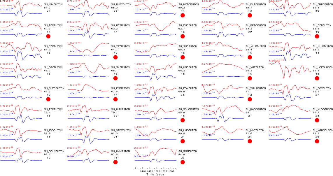
| SH-wave T component |
|
| Observed (red) and predicted seismograms (blue) ordered by increasing epicentral distance. Each pair of traces is annotated with the wave type and a station identifier (station, network, and channel id's), epicentral distance in degrees, source-to-station azimuth in degrees. Each seismogram pair is plotted with the same scale and the peak amplitudes in meters are shown above to the left of each trace. The optimal time shift between the observed first arrival and the predicted first arrival (in seconds) is shown above the prediction on the right. Red circles flag seismograms with amplitude misfits of a factor of 2 or more. |
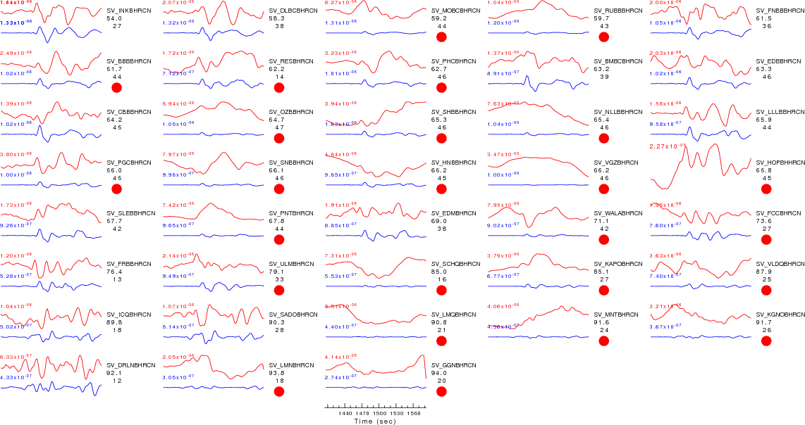
| SV-wave R component |
|
| Observed (red) and predicted seismograms (blue) ordered by increasing epicentral distance. Each pair of traces is annotated with the wave type and a station identifier (station, network, and channel id's), epicentral distance in degrees, source-to-station azimuth in degrees. Each seismogram pair is plotted with the same scale and the peak amplitudes in meters are shown above to the left of each trace. The optimal time shift between the observed first arrival and the predicted first arrival (in seconds) is shown above the prediction on the right. Red circles flag seismograms with amplitude misfits of a factor of 2 or more. |
BBBCNBHR BBBCNBHT BBBCNBHZ BMBCCNBHR BMBCCNBHT BMBCCNBHZ CBBCNBHR CBBCNBHT CBBCNBHZ DLBCCNBHR DLBCCNBHT DLBCCNBHZ DRLNCNBHR DRLNCNBHT DRLNCNBHZ EDBCNBHR EDBCNBHT EDBCNBHZ EDMCNBHR EDMCNBHT EDMCNBHZ FCCCNBHR FCCCNBHT FCCCNBHZ FNBBCNBHR FNBBCNBHT FNBBCNBHZ FRBCNBHR FRBCNBHT FRBCNBHZ GACCNEHZ GGNCNBHR GGNCNBHT GGNCNBHZ HNBCNBHR HNBCNBHT HNBCNBHZ HOPBCNHHR HOPBCNHHT HOPBCNHHZ ICQCNBHR ICQCNBHT ICQCNBHZ INKCNBHR INKCNBHT INKCNBHZ KAPOCNBHR KAPOCNBHT KAPOCNBHZ KGNOCNBHR KGNOCNBHT KGNOCNBHZ LLLBCNBHR LLLBCNBHT LLLBCNBHZ LMNCNBHR LMNCNBHT LMNCNBHZ LMQCNBHR LMQCNBHT LMQCNBHZ MNTCNBHR MNTCNBHT MNTCNBHZ MOBCCNBHR MOBCCNBHT MOBCCNBHZ NLLBCNBHR NLLBCNBHT NLLBCNBHZ OZBCNBHR OZBCNBHT OZBCNBHZ PGCCNBHR PGCCNBHT PGCCNBHZ PHCCNBHR PHCCNBHT PHCCNBHZ PNTCNBHR PNTCNBHT PNTCNBHZ RESCNBHR RESCNBHT RESCNBHZ RUBBCNBHR RUBBCNBHT RUBBCNBHZ SADOCNBHR SADOCNBHT SADOCNBHZ SCHQCNBHR SCHQCNBHT SCHQCNBHZ SHBCNBHR SHBCNBHT SHBCNBHZ SLEBCNBHR SLEBCNBHT SLEBCNBHZ SNBCNBHR SNBCNBHT SNBCNBHZ ULMCNBHR ULMCNBHT ULMCNBHZ VGZCNBHR VGZCNBHT VGZCNBHZ VLDQCNBHR VLDQCNBHT VLDQCNBHZ WALACNBHR WALACNBHT WALACNBHZ
Starting Processing         : Thu Dec 6 15:25:19 UTC 2007
Unpacking SEED volume       : Thu Dec 6 15:25:20 UTC 2007
Starting deconvolution      : Thu Dec 6 15:25:20 UTC 2007
Starting trace rotation     : Thu Dec 6 15:28:07 UTC 2007
Starting distance selection : Thu Dec 6 15:28:39 UTC 2007
Starting trace QC           : Thu Dec 6 15:28:55 UTC 2007
Starting synthetic          : Thu Dec 6 15:28:55 UTC 2007
Starting documentation      : Thu Dec 6 15:35:18 UTC 2007
Processing Completion       : Thu Dec 6 15:35:28 UTC 2007