Location

2013/11/27 04:13:38 40.878 27.884 9.6 4.5 TR

Arrival Times (from USGS)

Felt Map

Focal Mechanism

USGS/SLU Moment Tensor Solution ENS 2013/11/27 04:13:38:0 40.88 27.88 9.6 4.5 TR Stations used: KO.BALB KO.EDRB KO.EZN KO.GADA KO.GEMT KO.ISK KO.KLYT KO.RKY KO.YLV Filtering commands used: hp c 0.02 n 3 lp c 0.05 n 3 Best Fitting Double Couple Mo = 1.15e+23 dyne-cm Mw = 4.64 Z = 17 km Plane Strike Dip Rake NP1 353 80 170 NP2 85 80 10 Principal Axes: Axis Value Plunge Azimuth T 1.15e+23 14 309 N 0.00e+00 76 130 P -1.15e+23 0 39 Moment Tensor: (dyne-cm) Component Value Mxx -2.61e+22 Mxy -1.09e+23 Mxz 1.70e+22 Myy 1.93e+22 Myz -2.12e+22 Mzz 6.82e+21 #####--------- ##########------------ #############------------- P ############------------ ## T ############----------------- ### #############----------------- ####################------------------ ######################------------------ ######################------------------ #######################------------------- #######################----------------### ########################---------######### -------###########------################## -----------------------################# -----------------------################# ----------------------################ ---------------------############### --------------------############## ------------------############ -----------------########### --------------######## ----------#### Global CMT Convention Moment Tensor: R T P 6.82e+21 1.70e+22 2.12e+22 1.70e+22 -2.61e+22 1.09e+23 2.12e+22 1.09e+23 1.93e+22 Details of the solution is found at http://www.eas.slu.edu/eqc/eqc_mt/MECH.TR/20131127041338/index.html

Preferred Solution

The preferred solution from an analysis of the surface-wave spectral amplitude radiation pattern, waveform inversion and first motion observations is

      STK = 85
      DIP = 80
     RAKE = 10
       MW = 4.64
       HS = 17.0

The waveform inversion is preferred.

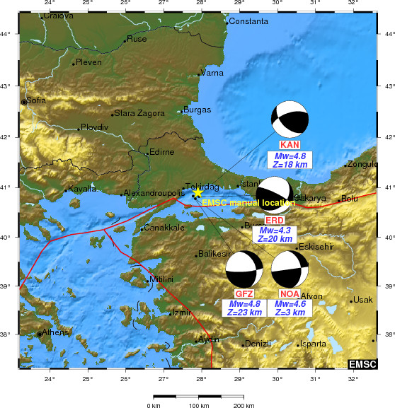
Moment Tensor Comparison

The following compares this source inversion to others

SLU EMSC

USGS/SLU Moment Tensor Solution ENS 2013/11/27 04:13:38:0 40.88 27.88 9.6 4.5 TR Stations used: KO.BALB KO.EDRB KO.EZN KO.GADA KO.GEMT KO.ISK KO.KLYT KO.RKY KO.YLV Filtering commands used: hp c 0.02 n 3 lp c 0.05 n 3 Best Fitting Double Couple Mo = 1.15e+23 dyne-cm Mw = 4.64 Z = 17 km Plane Strike Dip Rake NP1 353 80 170 NP2 85 80 10 Principal Axes: Axis Value Plunge Azimuth T 1.15e+23 14 309 N 0.00e+00 76 130 P -1.15e+23 0 39 Moment Tensor: (dyne-cm) Component Value Mxx -2.61e+22 Mxy -1.09e+23 Mxz 1.70e+22 Myy 1.93e+22 Myz -2.12e+22 Mzz 6.82e+21 #####--------- ##########------------ #############------------- P ############------------ ## T ############----------------- ### #############----------------- ####################------------------ ######################------------------ ######################------------------ #######################------------------- #######################----------------### ########################---------######### -------###########------################## -----------------------################# -----------------------################# ----------------------################ ---------------------############### --------------------############## ------------------############ -----------------########### --------------######## ----------#### Global CMT Convention Moment Tensor: R T P 6.82e+21 1.70e+22 2.12e+22 1.70e+22 -2.61e+22 1.09e+23 2.12e+22 1.09e+23 1.93e+22 Details of the solution is found at http://www.eas.slu.edu/eqc/eqc_mt/MECH.TR/20131127041338/index.html

Waveform Inversion

The focal mechanism was determined using broadband seismic waveforms. The location of the event and the and stations used for the waveform inversion are shown in the next figure.

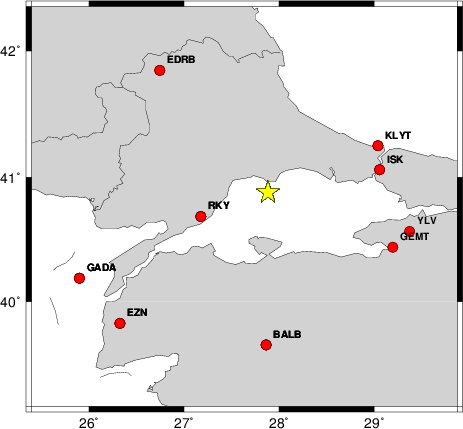
Location of broadband stations used for waveform inversion

The program wvfgrd96 was used with good traces observed at short distance to determine the focal mechanism, depth and seismic moment. This technique requires a high quality signal and well determined velocity model for the Green functions. To the extent that these are the quality data, this type of mechanism should be preferred over the radiation pattern technique which requires the separate step of defining the pressure and tension quadrants and the correct strike.

The observed and predicted traces are filtered using the following gsac commands:

hp c 0.02 n 3
lp c 0.05 n 3

The results of this grid search from 0.5 to 19 km depth are as follow:

           DEPTH  STK   DIP  RAKE   MW    FIT
WVFGRD96    0.5   265    70    20   4.20 0.1919
WVFGRD96    1.0   265    85     5   4.22 0.2098
WVFGRD96    2.0    85    70    15   4.34 0.2869
WVFGRD96    3.0    85    75    10   4.38 0.3201
WVFGRD96    4.0    85    70     5   4.42 0.3501
WVFGRD96    5.0    85    70     5   4.45 0.3791
WVFGRD96    6.0    85    70    10   4.48 0.4043
WVFGRD96    7.0    85    75    10   4.50 0.4292
WVFGRD96    8.0    85    70    10   4.53 0.4525
WVFGRD96    9.0    85    75    10   4.55 0.4687
WVFGRD96   10.0    85    75    10   4.57 0.4814
WVFGRD96   11.0    85    75    10   4.58 0.4909
WVFGRD96   12.0    85    85    15   4.60 0.4988
WVFGRD96   13.0    85    80    10   4.61 0.5045
WVFGRD96   14.0    85    80    10   4.62 0.5081
WVFGRD96   15.0    85    80    10   4.62 0.5113
WVFGRD96   16.0    85    80    10   4.63 0.5129
WVFGRD96   17.0    85    80    10   4.64 0.5133
WVFGRD96   18.0    85    80    10   4.65 0.5129
WVFGRD96   19.0    85    80    10   4.66 0.5121
WVFGRD96   20.0    85    80    10   4.66 0.5114
WVFGRD96   21.0    85    80    15   4.68 0.5102
WVFGRD96   22.0    85    80    10   4.68 0.5086
WVFGRD96   23.0    85    80    10   4.68 0.5063
WVFGRD96   24.0    85    80    10   4.69 0.5036
WVFGRD96   25.0    85    85    15   4.71 0.5006
WVFGRD96   26.0    85    85    15   4.71 0.4972
WVFGRD96   27.0    85    85    15   4.72 0.4934
WVFGRD96   28.0    85    85    15   4.73 0.4891
WVFGRD96   29.0    85    85    15   4.73 0.4844

The best solution is

WVFGRD96   17.0    85    80    10   4.64 0.5133

The mechanism correspond to the best fit is

Figure 1. Waveform inversion focal mechanism

The best fit as a function of depth is given in the following figure:

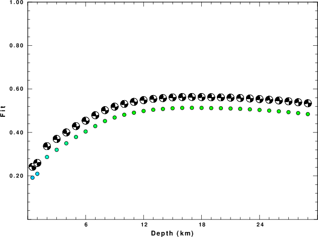
Figure 2. Depth sensitivity for waveform mechanism

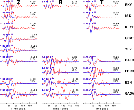
The comparison of the observed and predicted waveforms is given in the next figure. The red traces are the observed and the blue are the predicted. Each observed-predicted component is plotted to the same scale and peak amplitudes are indicated by the numbers to the left of each trace. A pair of numbers is given in black at the right of each predicted traces. The upper number it the time shift required for maximum correlation between the observed and predicted traces. This time shift is required because the synthetics are not computed at exactly the same distance as the observed and because the velocity model used in the predictions may not be perfect. A positive time shift indicates that the prediction is too fast and should be delayed to match the observed trace (shift to the right in this figure). A negative value indicates that the prediction is too slow. The lower number gives the percentage of variance reduction to characterize the individual goodness of fit (100% indicates a perfect fit).

The bandpass filter used in the processing and for the display was

hp c 0.02 n 3
lp c 0.05 n 3

Figure 3. Waveform comparison for selected depth. Red: observed; Blue - predicted. The time shift with respect to the model prediction is indicated. The percent of fit is also indicated.

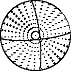
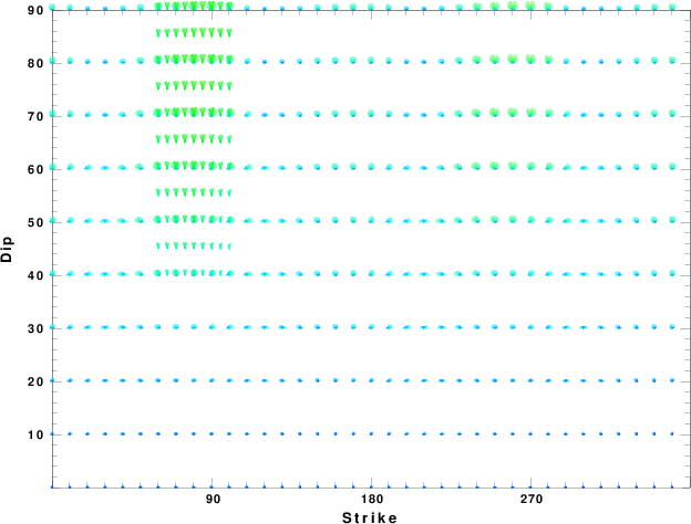
Focal mechanism sensitivity at the preferred depth. The red color indicates a very good fit to thewavefroms. Each solution is plotted as a vector at a given value of strike and dip with the angle of the vector representing the rake angle, measured, with respect to the upward vertical (N) in the figure.

Discussion

The Future

Should the national backbone of the USGS Advanced National Seismic System (ANSS) be implemented with an interstation separation of 300 km, it is very likely that an earthquake such as this would have been recorded at distances on the order of 100-200 km. This means that the closest station would have information on source depth and mechanism that was lacking here.

Acknowledgements

Dr. Harley Benz, USGS, provided the USGS USNSN digital data. The digital data used in this study were provided by Natural Resources Canada through their AUTODRM site http://www.seismo.nrcan.gc.ca/nwfa/autodrm/autodrm_req_e.php, and IRIS using their BUD interface.

Thanks also to the many seismic network operators whose dedication make this effort possible: University of Alaska, University of Washington, Oregon State University, University of Utah, Montana Bureas of Mines, UC Berkely, Caltech, UC San Diego, Saint L ouis University, Universityof Memphis, Lamont Doehrty Earth Observatory, Boston College, the Iris stations and the Transportable Array of EarthScope.

Velocity Model

The WUS used for the waveform synthetic seismograms and for the surface wave eigenfunctions and dispersion is as follows:

MODEL.01
Model after     8 iterations
ISOTROPIC
KGS
FLAT EARTH
1-D
CONSTANT VELOCITY
LINE08
LINE09
LINE10
LINE11
      H(KM)   VP(KM/S)   VS(KM/S) RHO(GM/CC)         QP         QS       ETAP       ETAS      FREFP      FREFS
     1.9000     3.4065     2.0089     2.2150  0.302E-02  0.679E-02   0.00       0.00       1.00       1.00    
     6.1000     5.5445     3.2953     2.6089  0.349E-02  0.784E-02   0.00       0.00       1.00       1.00    
    13.0000     6.2708     3.7396     2.7812  0.212E-02  0.476E-02   0.00       0.00       1.00       1.00    
    19.0000     6.4075     3.7680     2.8223  0.111E-02  0.249E-02   0.00       0.00       1.00       1.00    
     0.0000     7.9000     4.6200     3.2760  0.164E-10  0.370E-10   0.00       0.00       1.00       1.00

Quality Control

Here we tabulate the reasons for not using certain digital data sets

The following stations did not have a valid response files:

DATE=Wed Nov 27 16:10:09 CST 2013

Last Changed 2013/11/27