Location

2011/08/16 07:53:30 39.0800 35.9000 5.0 4.50 Turkey

Arrival Times (from USGS)

Felt Map

Focal Mechanism

USGS/SLU Moment Tensor Solution ENS 2011/08/16 07:53:30:0 39.08 35.90 5.0 4.5 Turkey Stations used: KO.BNN KO.BZK KO.CEYT KO.CORM KO.DARE KO.GAZ KO.HDMB KO.HRTX KO.IKL KO.KMRS KO.KONT KO.KOZT KO.KTUT KO.KVT KO.LADK KO.LEF KO.LFK KO.LOD KO.PTK KO.RSDY KO.SARI KO.SHUT KO.SILT KO.SPNC KO.SULT KO.SUTC KO.SVSK KO.URFA KO.VRTB Filtering commands used: hp c 0.02 n 3 lp c 0.06 n 3 Best Fitting Double Couple Mo = 1.50e+22 dyne-cm Mw = 4.05 Z = 13 km Plane Strike Dip Rake NP1 60 65 -30 NP2 164 63 -152 Principal Axes: Axis Value Plunge Azimuth T 1.50e+22 1 112 N 0.00e+00 52 204 P -1.50e+22 38 21 Moment Tensor: (dyne-cm) Component Value Mxx -5.87e+21 Mxy -8.35e+21 Mxz -6.90e+21 Myy 1.16e+22 Myz -2.34e+21 Mzz -5.73e+21 #------------- ####------------------ #######--------------------- #######----------- --------- #########----------- P ----------- ##########----------- ------------ ###########-------------------------## ############------------------------#### ############-----------------------##### #############---------------------######## ##############-------------------######### ##############-----------------########### ###############-------------############## ##############-----------############### ###############------################ ###############-#################### T #########------#################### ---------------################### --------------################ ---------------############# --------------######## ------------## Global CMT Convention Moment Tensor: R T P -5.73e+21 -6.90e+21 2.34e+21 -6.90e+21 -5.87e+21 8.35e+21 2.34e+21 8.35e+21 1.16e+22 Details of the solution is found at http://www.eas.slu.edu/eqc/eqc_mt/MECH.TR/20110816075330/index.html

Preferred Solution

The preferred solution from an analysis of the surface-wave spectral amplitude radiation pattern, waveform inversion and first motion observations is

      STK = 60
      DIP = 65
     RAKE = -30
       MW = 4.05
       HS = 13.0

The waveform inversion is preferred.

Moment Tensor Comparison

The following compares this source inversion to others

SLU

USGS/SLU Moment Tensor Solution ENS 2011/08/16 07:53:30:0 39.08 35.90 5.0 4.5 Turkey Stations used: KO.BNN KO.BZK KO.CEYT KO.CORM KO.DARE KO.GAZ KO.HDMB KO.HRTX KO.IKL KO.KMRS KO.KONT KO.KOZT KO.KTUT KO.KVT KO.LADK KO.LEF KO.LFK KO.LOD KO.PTK KO.RSDY KO.SARI KO.SHUT KO.SILT KO.SPNC KO.SULT KO.SUTC KO.SVSK KO.URFA KO.VRTB Filtering commands used: hp c 0.02 n 3 lp c 0.06 n 3 Best Fitting Double Couple Mo = 1.50e+22 dyne-cm Mw = 4.05 Z = 13 km Plane Strike Dip Rake NP1 60 65 -30 NP2 164 63 -152 Principal Axes: Axis Value Plunge Azimuth T 1.50e+22 1 112 N 0.00e+00 52 204 P -1.50e+22 38 21 Moment Tensor: (dyne-cm) Component Value Mxx -5.87e+21 Mxy -8.35e+21 Mxz -6.90e+21 Myy 1.16e+22 Myz -2.34e+21 Mzz -5.73e+21 #------------- ####------------------ #######--------------------- #######----------- --------- #########----------- P ----------- ##########----------- ------------ ###########-------------------------## ############------------------------#### ############-----------------------##### #############---------------------######## ##############-------------------######### ##############-----------------########### ###############-------------############## ##############-----------############### ###############------################ ###############-#################### T #########------#################### ---------------################### --------------################ ---------------############# --------------######## ------------## Global CMT Convention Moment Tensor: R T P -5.73e+21 -6.90e+21 2.34e+21 -6.90e+21 -5.87e+21 8.35e+21 2.34e+21 8.35e+21 1.16e+22 Details of the solution is found at http://www.eas.slu.edu/eqc/eqc_mt/MECH.TR/20110816075330/index.html

Waveform Inversion

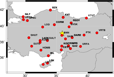
The focal mechanism was determined using broadband seismic waveforms. The location of the event and the and stations used for the waveform inversion are shown in the next figure.

Location of broadband stations used for waveform inversion

The program wvfgrd96 was used with good traces observed at short distance to determine the focal mechanism, depth and seismic moment. This technique requires a high quality signal and well determined velocity model for the Green functions. To the extent that these are the quality data, this type of mechanism should be preferred over the radiation pattern technique which requires the separate step of defining the pressure and tension quadrants and the correct strike.

The observed and predicted traces are filtered using the following gsac commands:

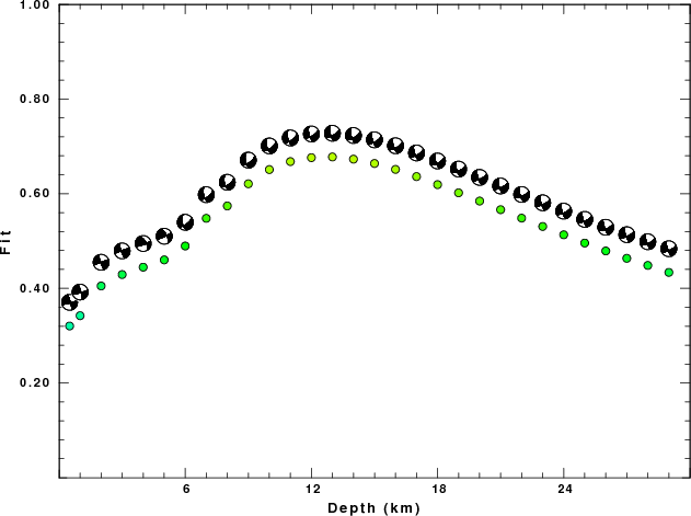
hp c 0.02 n 3
lp c 0.06 n 3

The results of this grid search from 0.5 to 19 km depth are as follow:

           DEPTH  STK   DIP  RAKE   MW    FIT
WVFGRD96    0.5    75    80    10   3.64 0.3205
WVFGRD96    1.0    75    80    10   3.68 0.3423
WVFGRD96    2.0    70    90    -5   3.76 0.4051
WVFGRD96    3.0   250    85    10   3.81 0.4292
WVFGRD96    4.0    70    75    35   3.87 0.4448
WVFGRD96    5.0    65    85    30   3.88 0.4602
WVFGRD96    6.0    55    65   -40   3.93 0.4896
WVFGRD96    7.0    55    60   -35   3.96 0.5480
WVFGRD96    8.0    55    60   -40   4.01 0.5742
WVFGRD96    9.0    55    60   -40   4.03 0.6210
WVFGRD96   10.0    55    60   -35   4.03 0.6510
WVFGRD96   11.0    55    60   -35   4.04 0.6679
WVFGRD96   12.0    60    65   -30   4.05 0.6763
WVFGRD96   13.0    60    65   -30   4.05 0.6777
WVFGRD96   14.0    60    65   -30   4.05 0.6730
WVFGRD96   15.0    60    65   -25   4.06 0.6639
WVFGRD96   16.0    60    65   -25   4.06 0.6514
WVFGRD96   17.0    60    65   -25   4.06 0.6362
WVFGRD96   18.0    60    65   -25   4.06 0.6192
WVFGRD96   19.0    65    70   -25   4.07 0.6020
WVFGRD96   20.0    65    70   -20   4.08 0.5845
WVFGRD96   21.0    65    70   -20   4.08 0.5663
WVFGRD96   22.0    65    70   -20   4.09 0.5484
WVFGRD96   23.0    65    70   -20   4.09 0.5308
WVFGRD96   24.0    65    70   -20   4.09 0.5132
WVFGRD96   25.0    65    70   -20   4.09 0.4958
WVFGRD96   26.0    65    70   -15   4.10 0.4791
WVFGRD96   27.0    65    70   -15   4.10 0.4635
WVFGRD96   28.0    65    70   -15   4.11 0.4485
WVFGRD96   29.0    65    70   -15   4.11 0.4338

The best solution is

WVFGRD96   13.0    60    65   -30   4.05 0.6777

The mechanism correspond to the best fit is

Figure 1. Waveform inversion focal mechanism

The best fit as a function of depth is given in the following figure:

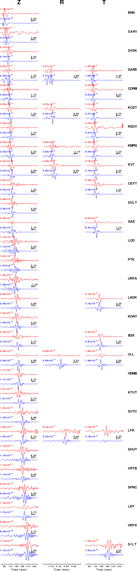
Figure 2. Depth sensitivity for waveform mechanism

The comparison of the observed and predicted waveforms is given in the next figure. The red traces are the observed and the blue are the predicted. Each observed-predicted component is plotted to the same scale and peak amplitudes are indicated by the numbers to the left of each trace. A pair of numbers is given in black at the right of each predicted traces. The upper number it the time shift required for maximum correlation between the observed and predicted traces. This time shift is required because the synthetics are not computed at exactly the same distance as the observed and because the velocity model used in the predictions may not be perfect. A positive time shift indicates that the prediction is too fast and should be delayed to match the observed trace (shift to the right in this figure). A negative value indicates that the prediction is too slow. The lower number gives the percentage of variance reduction to characterize the individual goodness of fit (100% indicates a perfect fit).

The bandpass filter used in the processing and for the display was

hp c 0.02 n 3
lp c 0.06 n 3

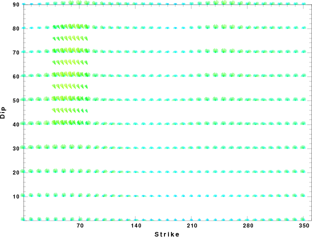
Figure 3. Waveform comparison for selected depth

Focal mechanism sensitivity at the preferred depth. The red color indicates a very good fit to thewavefroms. Each solution is plotted as a vector at a given value of strike and dip with the angle of the vector representing the rake angle, measured, with respect to the upward vertical (N) in the figure.

A check on the assumed source location is possible by looking at the time shifts between the observed and predicted traces. The time shifts for waveform matching arise for several reasons:

The origin time and epicentral distance are incorrect
The velocity model used for the inversion is incorrect
The velocity model used to define the P-arrival time is not the same as the velocity model used for the waveform inversion (assuming that the initial trace alignment is based on the P arrival time)

Assuming only a mislocation, the time shifts are fit to a functional form:

 Time_shift = A + B cos Azimuth + C Sin Azimuth

The time shifts for this inversion lead to the next figure:

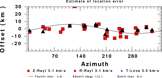
The derived shift in origin time and epicentral coordinates are given at the bottom of the figure.

Discussion

Velocity Model

The WUS used for the waveform synthetic seismograms and for the surface wave eigenfunctions and dispersion is as follows:

MODEL.01
Model after     8 iterations
ISOTROPIC
KGS
FLAT EARTH
1-D
CONSTANT VELOCITY
LINE08
LINE09
LINE10
LINE11
      H(KM)   VP(KM/S)   VS(KM/S) RHO(GM/CC)         QP         QS       ETAP       ETAS      FREFP      FREFS
     1.9000     3.4065     2.0089     2.2150  0.302E-02  0.679E-02   0.00       0.00       1.00       1.00    
     6.1000     5.5445     3.2953     2.6089  0.349E-02  0.784E-02   0.00       0.00       1.00       1.00    
    13.0000     6.2708     3.7396     2.7812  0.212E-02  0.476E-02   0.00       0.00       1.00       1.00    
    19.0000     6.4075     3.7680     2.8223  0.111E-02  0.249E-02   0.00       0.00       1.00       1.00    
     0.0000     7.9000     4.6200     3.2760  0.164E-10  0.370E-10   0.00       0.00       1.00       1.00

Quality Control

Here we tabulate the reasons for not using certain digital data sets

The following stations did not have a valid response files:

DATE=Tue Aug 16 20:16:22 CDT 2011

Last Changed 2011/08/16