Location
KANDİLLİ Observ atory Location
Tarih      Saat      Enlem(N)  Boylam(E) Derinlik(km)  MD   ML   MS    Yer                                             Çözüm Niteliği
---------- --------  --------  -------   ----------    ------------    --------------                                  --------------
2011.05.19 23:15:22  39.1490   29.1025        7.0      -.-  5.9  -.-   SİMAV (KÜTAHYA)                                   İlksel
USGS Location
2011/05/19 20:15:23 39.115 29.124 4.6 6.00 Turkey
Arrival Times (from USGS)
Arrival time list
Felt Map
USGS Felt map for this earthquake
USGS Felt reports page for
Focal Mechanism
 USGS/SLU Moment Tensor Solution
 ENS  2011/05/19 20:15:23:0  39.12   29.12   4.6 6.0 Turkey

 Stations used:
   GE.ISP KO.ADVT KO.ARMT KO.BALB KO.BCK KO.BGKT KO.CAVI
   KO.CTKS KO.EDC KO.ERIK KO.EZN KO.GELI KO.GEMT KO.GLHS
   KO.GULT KO.HRTX KO.ISK KO.KCTX KO.KLYT KO.KRBG KO.KULA
   KO.LADK KO.LAP KO.MDNY KO.MDUB KO.MRMT KO.RKY KO.SILT
   KO.SPNC KO.SUTC KO.SVRH KO.TKR KO.YER

 Filtering commands used:
   hp c 0.02 n 3
   lp c 0.10 n 3

 Best Fitting Double Couple
  Mo = 5.13e+24 dyne-cm
  Mw = 5.74
  Z  = 13 km
  Plane   Strike  Dip  Rake
   NP1      300    50   -60
   NP2       78    48   -121
  Principal Axes:
   Axis    Value   Plunge  Azimuth
    T   5.13e+24      1       9
    N   0.00e+00     23     100
    P  -5.13e+24     67     277

 Moment Tensor: (dyne-cm)
    Component   Value
       Mxx     4.98e+24
       Mxy     9.12e+23
       Mxz    -1.56e+23
       Myy    -6.08e+23
       Myz     1.81e+24
       Mzz    -4.37e+24


                     ######### T ##
                 #############   ######
              ############################
             ##############################
           ###-----------####################
          --------------------################
         -------------------------#############
        ----------------------------############
        -------------------------------#########
       --------------   ----------------########-
       -------------- P ------------------#####--
       --------------   -------------------###---
       ------------------------------------------
        ----------------------------------###---
        ##-----------------------------######---
         ####-----------------------##########-
          ########------------################
           ##################################
             ##############################
              ############################
                 ######################
                     ##############


 Global CMT Convention Moment Tensor:
      R          T          P
 -4.37e+24  -1.56e+23  -1.81e+24
 -1.56e+23   4.98e+24  -9.12e+23
 -1.81e+24  -9.12e+23  -6.08e+23


Details of the solution is found at

http://www.eas.slu.edu/Earthquake_Center/MECH.NA/20110519201523/index.html
|
Preferred Solution
The preferred solution from an analysis of the surface-wave spectral amplitude radiation pattern, waveform inversion and first motion observations is
      STK = 300
      DIP = 50
     RAKE = -60
       MW = 5.74
       HS = 13.0
The waveform inversion is preferred.
Moment Tensor Comparison
The following compares this source inversion to others
| SLU |
USGSMT |
 USGS/SLU Moment Tensor Solution
 ENS  2011/05/19 20:15:23:0  39.12   29.12   4.6 6.0 Turkey

 Stations used:
   GE.ISP KO.ADVT KO.ARMT KO.BALB KO.BCK KO.BGKT KO.CAVI
   KO.CTKS KO.EDC KO.ERIK KO.EZN KO.GELI KO.GEMT KO.GLHS
   KO.GULT KO.HRTX KO.ISK KO.KCTX KO.KLYT KO.KRBG KO.KULA
   KO.LADK KO.LAP KO.MDNY KO.MDUB KO.MRMT KO.RKY KO.SILT
   KO.SPNC KO.SUTC KO.SVRH KO.TKR KO.YER

 Filtering commands used:
   hp c 0.02 n 3
   lp c 0.10 n 3

 Best Fitting Double Couple
  Mo = 5.13e+24 dyne-cm
  Mw = 5.74
  Z  = 13 km
  Plane   Strike  Dip  Rake
   NP1      300    50   -60
   NP2       78    48   -121
  Principal Axes:
   Axis    Value   Plunge  Azimuth
    T   5.13e+24      1       9
    N   0.00e+00     23     100
    P  -5.13e+24     67     277

 Moment Tensor: (dyne-cm)
    Component   Value
       Mxx     4.98e+24
       Mxy     9.12e+23
       Mxz    -1.56e+23
       Myy    -6.08e+23
       Myz     1.81e+24
       Mzz    -4.37e+24


                     ######### T ##
                 #############   ######
              ############################
             ##############################
           ###-----------####################
          --------------------################
         -------------------------#############
        ----------------------------############
        -------------------------------#########
       --------------   ----------------########-
       -------------- P ------------------#####--
       --------------   -------------------###---
       ------------------------------------------
        ----------------------------------###---
        ##-----------------------------######---
         ####-----------------------##########-
          ########------------################
           ##################################
             ##############################
              ############################
                 ######################
                     ##############


 Global CMT Convention Moment Tensor:
      R          T          P
 -4.37e+24  -1.56e+23  -1.81e+24
 -1.56e+23   4.98e+24  -9.12e+23
 -1.81e+24  -9.12e+23  -6.08e+23


Details of the solution is found at

http://www.eas.slu.edu/Earthquake_Center/MECH.NA/20110519201523/index.html
|
USGS/SLU Regional Moment Solution
WESTERN TURKEY

11/05/19 20:15:24.42

Epicenter:  39.104   29.099
MW 5.8

USGS/SLU REGIONAL MOMENT TENSOR
Depth  11         No. of sta: 24
Moment Tensor;   Scale 10**17 Nm
  Mrr=-5.05       Mtt= 6.23
  Mpp=-1.17       Mrt= 2.07
  Mrp= 1.90       Mtp=-2.31
 Principal axes:
  T  Val=  7.08  Plg= 7  Azm= 14
  N       -0.62      27      280
  P       -6.46      62      118

Best Double Couple:Mo=6.8*10**17
 NP1:Strike=131 Dip=44 Slip= -50
 NP2:       262     58      -122
|
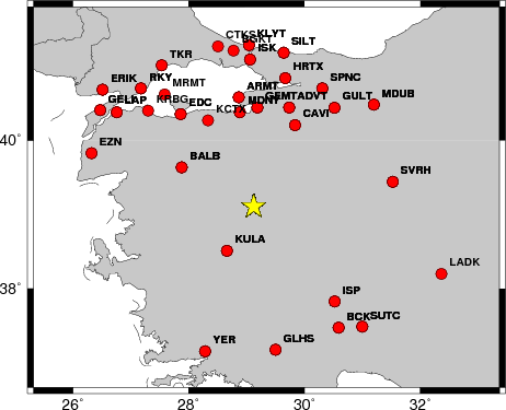
Waveform Inversion
The focal mechanism was determined using broadband seismic waveforms. The location of the event and the
and stations used for the waveform inversion are shown in the next figure.
|
|
Location of broadband stations used for waveform inversion
|
The program wvfgrd96 was used with good traces observed at short distance to determine the focal mechanism, depth and seismic moment. This technique requires a high quality signal and well determined velocity model for the Green functions. To the extent that these are the quality data, this type of mechanism should be preferred over the radiation pattern technique which requires the separate step of defining the pressure and tension quadrants and the correct strike.
The observed and predicted traces are filtered using the following gsac commands:
hp c 0.02 n 3
lp c 0.10 n 3
The results of this grid search from 0.5 to 19 km depth are as follow:
           DEPTH  STK   DIP  RAKE   MW    FIT
WVFGRD96    0.5   280    50   -90   5.32 0.3150
WVFGRD96    1.0   275    45    90   5.35 0.2814
WVFGRD96    2.0   100    45    95   5.48 0.3420
WVFGRD96    3.0   120    25   -55   5.53 0.2784
WVFGRD96    4.0    25    15    20   5.53 0.3368
WVFGRD96    5.0   265    80    75   5.54 0.3985
WVFGRD96    6.0    30    20    30   5.55 0.4428
WVFGRD96    7.0   340    50    40   5.62 0.4743
WVFGRD96    8.0   265    75    75   5.65 0.4972
WVFGRD96    9.0   265    70    75   5.67 0.5109
WVFGRD96   10.0   345    50    45   5.73 0.5194
WVFGRD96   11.0   340    55    40   5.74 0.5215
WVFGRD96   12.0   300    50   -60   5.73 0.5213
WVFGRD96   13.0   300    50   -60   5.74 0.5280
WVFGRD96   14.0   305    55   -55   5.76 0.5272
WVFGRD96   15.0   125    55   -50   5.77 0.5223
WVFGRD96   16.0   125    55   -50   5.78 0.5118
WVFGRD96   17.0   125    55   -50   5.79 0.4969
WVFGRD96   18.0   135    45   -35   5.79 0.4796
WVFGRD96   19.0   140    40   -30   5.79 0.4616
WVFGRD96   20.0   145    40   -20   5.80 0.4443
WVFGRD96   21.0   145    40   -20   5.81 0.4281
WVFGRD96   22.0   145    40   -20   5.82 0.4101
WVFGRD96   23.0   150    40   -10   5.83 0.3932
WVFGRD96   24.0   150    40   -10   5.83 0.3764
WVFGRD96   25.0   150    35   -10   5.83 0.3602
WVFGRD96   26.0   150    35   -10   5.84 0.3445
WVFGRD96   27.0   150    35   -10   5.85 0.3294
WVFGRD96   28.0   150    35   -10   5.85 0.3144
WVFGRD96   29.0   150    35   -10   5.86 0.2995
The best solution is
WVFGRD96 13.0 300 50 -60 5.74 0.5280
The mechanism correspond to the best fit is
|
|
Figure 1. Waveform inversion focal mechanism
|
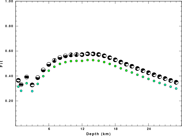
The best fit as a function of depth is given in the following figure:
|
|
Figure 2. Depth sensitivity for waveform mechanism
|
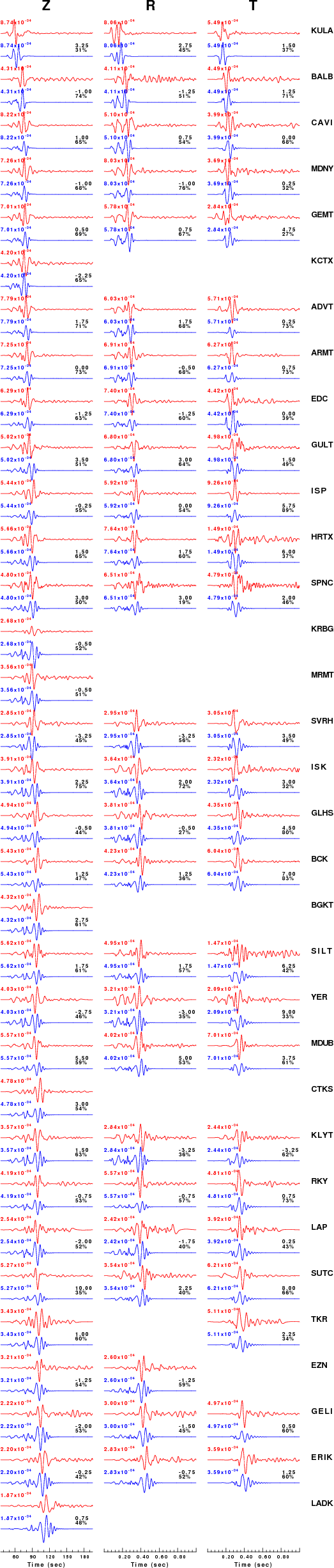
The comparison of the observed and predicted waveforms is given in the next figure. The red traces are the observed and the blue are the predicted.
Each observed-predicted component is plotted to the same scale and peak amplitudes are indicated by the numbers to the left of each trace. A pair of numbers is given in black at the right of each predicted traces. The upper number it the time shift required for maximum correlation between the observed and predicted traces. This time shift is required because the synthetics are not computed at exactly the same distance as the observed and because the velocity model used in the predictions may not be perfect.
A positive time shift indicates that the prediction is too fast and should be delayed to match the observed trace (shift to the right in this figure). A negative value indicates that the prediction is too slow. The lower number gives the percentage of variance reduction to characterize the individual goodness of fit (100% indicates a perfect fit).
The bandpass filter used in the processing and for the display was
hp c 0.02 n 3
lp c 0.10 n 3
|
|
Figure 3. Waveform comparison for selected depth
|
|
|
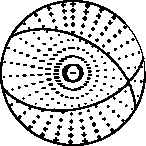
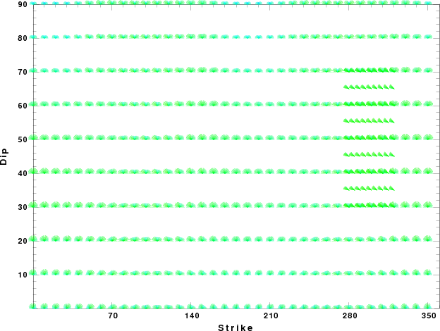
Focal mechanism sensitivity at the preferred depth. The red color indicates a very good fit to thewavefroms.
Each solution is plotted as a vector at a given value of strike and dip with the angle of the vector representing the rake angle, measured, with respect to the upward vertical (N) in the figure.
|
A check on the assumed source location is possible by looking at the time shifts between the observed and predicted traces. The time shifts for waveform matching arise for several reasons:
- The origin time and epicentral distance are incorrect
- The velocity model used for the inversion is incorrect
- The velocity model used to define the P-arrival time is not the
same as the velocity model used for the waveform inversion
(assuming that the initial trace alignment is based on the
P arrival time)
Assuming only a mislocation, the time shifts are fit to a functional form:
Time_shift = A + B cos Azimuth + C Sin Azimuth
The time shifts for this inversion lead to the next figure:
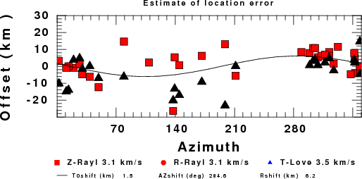
The derived shift in origin time and epicentral coordinates are given at the bottom of the figure.
Discussion
Velocity Model
The WUS used for the waveform synthetic seismograms and for the surface wave eigenfunctions and dispersion is as follows:
MODEL.01
Model after     8 iterations
ISOTROPIC
KGS
FLAT EARTH
1-D
CONSTANT VELOCITY
LINE08
LINE09
LINE10
LINE11
      H(KM)   VP(KM/S)   VS(KM/S) RHO(GM/CC)         QP         QS       ETAP       ETAS      FREFP      FREFS
     1.9000     3.4065     2.0089     2.2150  0.302E-02  0.679E-02   0.00       0.00       1.00       1.00
     6.1000     5.5445     3.2953     2.6089  0.349E-02  0.784E-02   0.00       0.00       1.00       1.00
    13.0000     6.2708     3.7396     2.7812  0.212E-02  0.476E-02   0.00       0.00       1.00       1.00
    19.0000     6.4075     3.7680     2.8223  0.111E-02  0.249E-02   0.00       0.00       1.00       1.00
     0.0000     7.9000     4.6200     3.2760  0.164E-10  0.370E-10   0.00       0.00       1.00       1.00
Quality Control
Here we tabulate the reasons for not using certain digital data sets
The following stations did not have a valid response files:
DATE=Thu May 19 17:19:00 CDT 2011
Last Changed 2011/05/19