2010/03/24 14:11:33 38.786 40.211 18.7 4.90 Turkey
USGS Felt map for this earthquake
 USGS/SLU Moment Tensor Solution
 ENS  2010/03/24 14:11:33:8  38.79   40.21  18.7 4.9 Turkey

 Stations used:
   KO.AGRB KO.BAYT KO.BCA KO.CEYT KO.CLDR KO.CORM KO.CUKT
   KO.DARE KO.DIKM KO.ERZN KO.ESPY KO.ILIC KO.KARA KO.KARS
   KO.KOZT KO.KTUT KO.KVT KO.RSDY KO.SIRT KO.SVSK KO.URFA
   KO.VANB KO.VRTB

 Filtering commands used:
   hp c 0.02 n 3
   lp c 0.05 n 3

 Best Fitting Double Couple
  Mo = 2.63e+23 dyne-cm
  Mw = 4.88
  Z  = 13 km
  Plane   Strike  Dip  Rake
   NP1      138    71   137
   NP2      245    50    25
  Principal Axes:
   Axis    Value   Plunge  Azimuth
    T   2.63e+23     43      94
    N   0.00e+00     44     299
    P  -2.63e+23     13     196

 Moment Tensor: (dyne-cm)
    Component   Value
       Mxx    -2.30e+23
       Mxy    -7.55e+22
       Mxz     4.73e+22
       Myy     1.20e+23
       Myz     1.47e+23
       Mzz     1.09e+23


                     --------------
                 ----------------------
              ----------------------------
             #-----------------------------
           ####------------------------------
          ######----------##################--
         #######------#########################
        #########--#############################
        #########--#############################
       ########-----#############################
       ######--------#################   ########
       #####----------################ T ########
       ####-------------##############   ########
        ##----------------######################
        ##------------------####################
         ---------------------#################
          ----------------------##############
           -----------------------###########
             -------------------------#####
              -------   ------------------
                 ---- P ---------------
                        -----------


 Global CMT Convention Moment Tensor:
      R          T          P
  1.09e+23   4.73e+22  -1.47e+23
  4.73e+22  -2.30e+23   7.55e+22
 -1.47e+23   7.55e+22   1.20e+23


Details of the solution is found at

http://www.eas.slu.edu/Earthquake_Center/MECH.NA/20100324141133/index.html
|
      STK = 245
      DIP = 50
     RAKE = 25
       MW = 4.88
       HS = 13.0
The waveform inversion is preferred.
The following compares this source inversion to others
 USGS/SLU Moment Tensor Solution
 ENS  2010/03/24 14:11:33:8  38.79   40.21  18.7 4.9 Turkey

 Stations used:
   KO.AGRB KO.BAYT KO.BCA KO.CEYT KO.CLDR KO.CORM KO.CUKT
   KO.DARE KO.DIKM KO.ERZN KO.ESPY KO.ILIC KO.KARA KO.KARS
   KO.KOZT KO.KTUT KO.KVT KO.RSDY KO.SIRT KO.SVSK KO.URFA
   KO.VANB KO.VRTB

 Filtering commands used:
   hp c 0.02 n 3
   lp c 0.05 n 3

 Best Fitting Double Couple
  Mo = 2.63e+23 dyne-cm
  Mw = 4.88
  Z  = 13 km
  Plane   Strike  Dip  Rake
   NP1      138    71   137
   NP2      245    50    25
  Principal Axes:
   Axis    Value   Plunge  Azimuth
    T   2.63e+23     43      94
    N   0.00e+00     44     299
    P  -2.63e+23     13     196

 Moment Tensor: (dyne-cm)
    Component   Value
       Mxx    -2.30e+23
       Mxy    -7.55e+22
       Mxz     4.73e+22
       Myy     1.20e+23
       Myz     1.47e+23
       Mzz     1.09e+23


                     --------------
                 ----------------------
              ----------------------------
             #-----------------------------
           ####------------------------------
          ######----------##################--
         #######------#########################
        #########--#############################
        #########--#############################
       ########-----#############################
       ######--------#################   ########
       #####----------################ T ########
       ####-------------##############   ########
        ##----------------######################
        ##------------------####################
         ---------------------#################
          ----------------------##############
           -----------------------###########
             -------------------------#####
              -------   ------------------
                 ---- P ---------------
                        -----------


 Global CMT Convention Moment Tensor:
      R          T          P
  1.09e+23   4.73e+22  -1.47e+23
  4.73e+22  -2.30e+23   7.55e+22
 -1.47e+23   7.55e+22   1.20e+23


Details of the solution is found at

http://www.eas.slu.edu/Earthquake_Center/MECH.NA/20100324141133/index.html
|
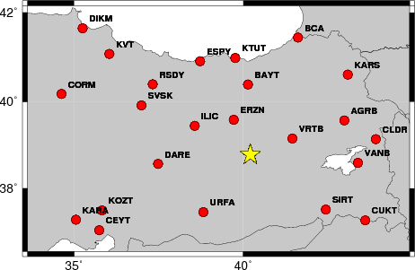
The focal mechanism was determined using broadband seismic waveforms. The location of the event and the and stations used for the waveform inversion are shown in the next figure.
|
|
|
|
The program wvfgrd96 was used with good traces observed at short distance to determine the focal mechanism, depth and seismic moment. This technique requires a high quality signal and well determined velocity model for the Green functions. To the extent that these are the quality data, this type of mechanism should be preferred over the radiation pattern technique which requires the separate step of defining the pressure and tension quadrants and the correct strike.
The observed and predicted traces are filtered using the following gsac commands:
hp c 0.02 n 3
lp c 0.05 n 3
The results of this grid search from 0.5 to 19 km depth are as follow:
           DEPTH  STK   DIP  RAKE   MW    FIT
WVFGRD96    0.5    50    65   -35   4.55 0.3385
WVFGRD96    1.0    55    85    -5   4.53 0.3549
WVFGRD96    2.0   230    65   -35   4.66 0.4242
WVFGRD96    3.0   230    55   -25   4.70 0.4471
WVFGRD96    4.0   230    45   -20   4.75 0.4714
WVFGRD96    5.0   235    40   -10   4.79 0.5029
WVFGRD96    6.0   235    40   -10   4.80 0.5278
WVFGRD96    7.0   245    45    15   4.80 0.5498
WVFGRD96    8.0   245    40    15   4.85 0.5638
WVFGRD96    9.0   245    40    15   4.86 0.5828
WVFGRD96   10.0   250    45    25   4.87 0.5979
WVFGRD96   11.0   250    45    30   4.88 0.6082
WVFGRD96   12.0   245    50    25   4.88 0.6131
WVFGRD96   13.0   245    50    25   4.88 0.6150
WVFGRD96   14.0   245    50    25   4.89 0.6133
WVFGRD96   15.0   245    50    20   4.89 0.6097
WVFGRD96   16.0   245    50    20   4.89 0.6042
WVFGRD96   17.0   245    55    20   4.89 0.5980
WVFGRD96   18.0   245    55    20   4.90 0.5906
WVFGRD96   19.0   245    55    20   4.90 0.5825
WVFGRD96   20.0   245    55    20   4.91 0.5733
WVFGRD96   21.0   245    55    20   4.92 0.5636
WVFGRD96   22.0   245    55    20   4.92 0.5532
WVFGRD96   23.0   245    55    20   4.92 0.5422
WVFGRD96   24.0   245    55    20   4.93 0.5309
WVFGRD96   25.0   245    55    15   4.93 0.5193
WVFGRD96   26.0   245    55    15   4.93 0.5077
WVFGRD96   27.0   155    80    35   4.93 0.5011
WVFGRD96   28.0   155    75    30   4.94 0.4959
WVFGRD96   29.0   330    85   -30   4.95 0.4881
The best solution is
WVFGRD96 13.0 245 50 25 4.88 0.6150
The mechanism correspond to the best fit is
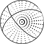
|
|
|
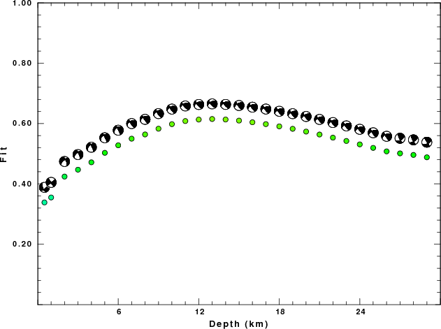
The best fit as a function of depth is given in the following figure:
|
|
|
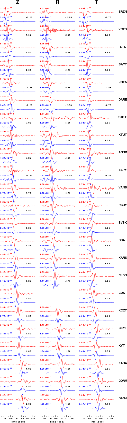
The comparison of the observed and predicted waveforms is given in the next figure. The red traces are the observed and the blue are the predicted. Each observed-predicted componnet is plotted to the same scale and peak amplitudes are indicated by the numbers to the left of each trace. The number in black at the rightr of each predicted traces it the time shift required for maximum correlation between the observed and predicted traces. This time shift is required because the synthetics are not computed at exactly the same distance as the observed and because the velocity model used in the predictions may not be perfect. A positive time shift indicates that the prediction is too fast and should be delayed to match the observed trace (shift to the right in this figure). A negative value indicates that the prediction is too slow. The bandpass filter used in the processing and for the display was
hp c 0.02 n 3
lp c 0.05 n 3
|
|
|
|
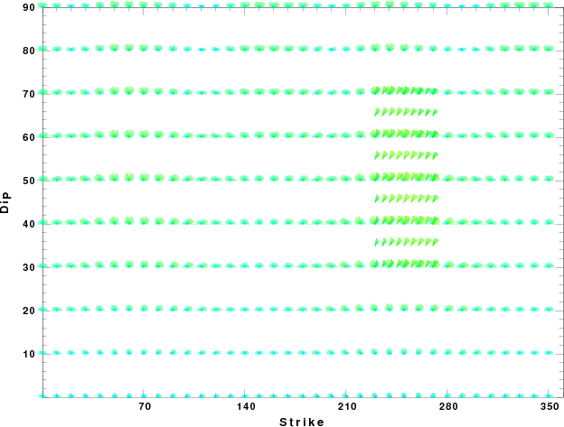
| Focal mechanism sensitivity at the preferred depth. The red color indicates a very good fit to thewavefroms. Each solution is plotted as a vector at a given value of strike and dip with the angle of the vector representing the rake angle, measured, with respect to the upward vertical (N) in the figure. |
The WUS used for the waveform synthetic seismograms and for the surface wave eigenfunctions and dispersion is as follows:
MODEL.01
Model after     8 iterations
ISOTROPIC
KGS
FLAT EARTH
1-D
CONSTANT VELOCITY
LINE08
LINE09
LINE10
LINE11
      H(KM)   VP(KM/S)   VS(KM/S) RHO(GM/CC)         QP         QS       ETAP       ETAS      FREFP      FREFS
     1.9000     3.4065     2.0089     2.2150  0.302E-02  0.679E-02   0.00       0.00       1.00       1.00
     6.1000     5.5445     3.2953     2.6089  0.349E-02  0.784E-02   0.00       0.00       1.00       1.00
    13.0000     6.2708     3.7396     2.7812  0.212E-02  0.476E-02   0.00       0.00       1.00       1.00
    19.0000     6.4075     3.7680     2.8223  0.111E-02  0.249E-02   0.00       0.00       1.00       1.00
     0.0000     7.9000     4.6200     3.2760  0.164E-10  0.370E-10   0.00       0.00       1.00       1.00
Here we tabulate the reasons for not using certain digital data sets
The following stations did not have a valid response files:
DATE=Wed Mar 24 20:40:31 CDT 2010