2009/06/17 04:29:18 36.1000 35.9300 20.0 4.60 Turkey
USGS Felt map for this earthquake
 USGS/SLU Moment Tensor Solution
 ENS  2009/06/17 04:29:18:0  36.10   35.93  20.0 4.6 Turkey

 Stations used:
   KO.BNN KO.DIKM KO.ESPY KO.KMRS KO.KRTS KO.KVT KO.PTK
   KO.URFA

 Filtering commands used:
   hp c 0.02 n 3
   lp c 0.05 n 3

 Best Fitting Double Couple
  Mo = 5.75e+22 dyne-cm
  Mw = 4.44
  Z  = 18 km
  Plane   Strike  Dip  Rake
   NP1       25    53   106
   NP2      180    40    70
  Principal Axes:
   Axis    Value   Plunge  Azimuth
    T   5.75e+22     76     347
    N   0.00e+00     13     196
    P  -5.75e+22      7     104

 Moment Tensor: (dyne-cm)
    Component   Value
       Mxx    -2.21e+15
       Mxy     1.27e+22
       Mxz     1.51e+22
       Myy    -5.33e+22
       Myz    -9.39e+21
       Mzz     5.33e+22


                     ----##########
                 ------###############-
              -------#################----
             -------###################----
           --------####################------
          --------#####################-------
         --------######################--------
        --------#######################---------
        --------##########   ##########---------
       ---------########## T ##########----------
       ---------##########   #########-----------
       ---------######################-----------
       ---------#####################--------   -
        --------####################--------- P
        --------###################----------
         --------#################-------------
          --------###############-------------
           --------############--------------
             -------#########--------------
              -------######---------------
                 ----------------------
                     ####----------


 Global CMT Convention Moment Tensor:
      R          T          P
  5.33e+22   1.51e+22   9.39e+21
  1.51e+22  -2.21e+15  -1.27e+22
  9.39e+21  -1.27e+22  -5.33e+22


Details of the solution is found at

http://www.eas.slu.edu/Earthquake_Center/MECH.NA/20090617042918/index.html
|
      STK = 180
      DIP = 40
     RAKE = 70
       MW = 4.44
       HS = 18.0
The waveform inversion is preferred.
The following compares this source inversion to others
 USGS/SLU Moment Tensor Solution
 ENS  2009/06/17 04:29:18:0  36.10   35.93  20.0 4.6 Turkey

 Stations used:
   KO.BNN KO.DIKM KO.ESPY KO.KMRS KO.KRTS KO.KVT KO.PTK
   KO.URFA

 Filtering commands used:
   hp c 0.02 n 3
   lp c 0.05 n 3

 Best Fitting Double Couple
  Mo = 5.75e+22 dyne-cm
  Mw = 4.44
  Z  = 18 km
  Plane   Strike  Dip  Rake
   NP1       25    53   106
   NP2      180    40    70
  Principal Axes:
   Axis    Value   Plunge  Azimuth
    T   5.75e+22     76     347
    N   0.00e+00     13     196
    P  -5.75e+22      7     104

 Moment Tensor: (dyne-cm)
    Component   Value
       Mxx    -2.21e+15
       Mxy     1.27e+22
       Mxz     1.51e+22
       Myy    -5.33e+22
       Myz    -9.39e+21
       Mzz     5.33e+22


                     ----##########
                 ------###############-
              -------#################----
             -------###################----
           --------####################------
          --------#####################-------
         --------######################--------
        --------#######################---------
        --------##########   ##########---------
       ---------########## T ##########----------
       ---------##########   #########-----------
       ---------######################-----------
       ---------#####################--------   -
        --------####################--------- P
        --------###################----------
         --------#################-------------
          --------###############-------------
           --------############--------------
             -------#########--------------
              -------######---------------
                 ----------------------
                     ####----------


 Global CMT Convention Moment Tensor:
      R          T          P
  5.33e+22   1.51e+22   9.39e+21
  1.51e+22  -2.21e+15  -1.27e+22
  9.39e+21  -1.27e+22  -5.33e+22


Details of the solution is found at

http://www.eas.slu.edu/Earthquake_Center/MECH.NA/20090617042918/index.html
|
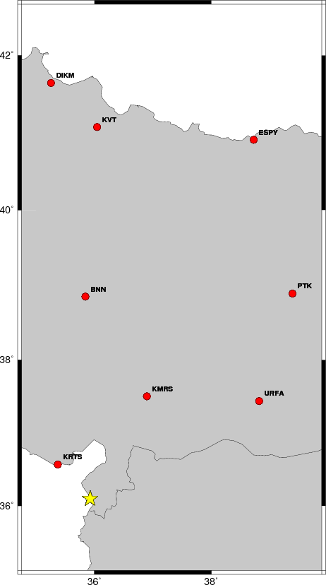
The focal mechanism was determined using broadband seismic waveforms. The location of the event and the and stations used for the waveform inversion are shown in the next figure.
|
|
|
|
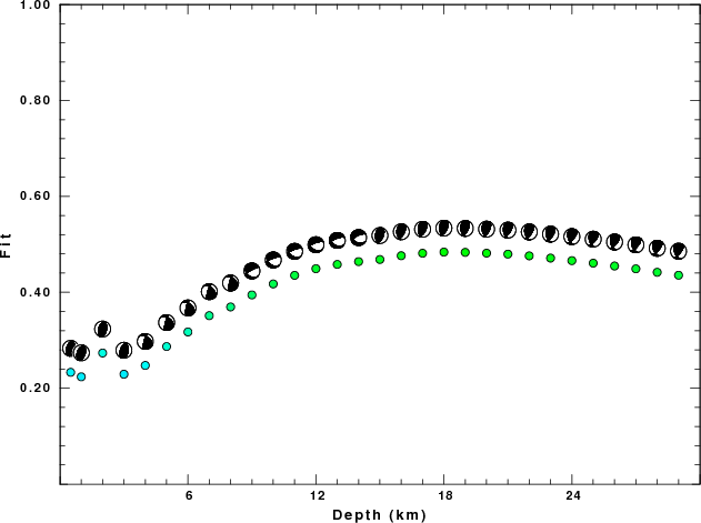
The program wvfgrd96 was used with good traces observed at short distance to determine the focal mechanism, depth and seismic moment. This technique requires a high quality signal and well determined velocity model for the Green functions. To the extent that these are the quality data, this type of mechanism should be preferred over the radiation pattern technique which requires the separate step of defining the pressure and tension quadrants and the correct strike.
The observed and predicted traces are filtered using the following gsac commands:
hp c 0.02 n 3
lp c 0.05 n 3
The results of this grid search from 0.5 to 19 km depth are as follow:
           DEPTH  STK   DIP  RAKE   MW    FIT
WVFGRD96    0.5    10    45    85   4.09 0.2332
WVFGRD96    1.0    15    45    85   4.12 0.2238
WVFGRD96    2.0    10    45    85   4.22 0.2734
WVFGRD96    3.0   200    50   100   4.24 0.2292
WVFGRD96    4.0   305    35    25   4.28 0.2475
WVFGRD96    5.0   305    35    25   4.30 0.2869
WVFGRD96    6.0   310    40    35   4.31 0.3173
WVFGRD96    7.0   310    40    30   4.31 0.3513
WVFGRD96    8.0   310    30    30   4.38 0.3694
WVFGRD96    9.0   130    30   -25   4.36 0.3945
WVFGRD96   10.0   130    35   -35   4.37 0.4174
WVFGRD96   11.0   125    35   -40   4.38 0.4353
WVFGRD96   12.0   125    35   -40   4.39 0.4492
WVFGRD96   13.0   120    35   -45   4.39 0.4581
WVFGRD96   14.0   115    35   -45   4.40 0.4640
WVFGRD96   15.0   185    40    75   4.44 0.4684
WVFGRD96   16.0   180    40    70   4.44 0.4762
WVFGRD96   17.0   180    40    70   4.44 0.4814
WVFGRD96   18.0   180    40    70   4.44 0.4838
WVFGRD96   19.0   175    40    65   4.44 0.4832
WVFGRD96   20.0   175    40    65   4.44 0.4816
WVFGRD96   21.0   175    40    60   4.45 0.4796
WVFGRD96   22.0   170    40    55   4.45 0.4759
WVFGRD96   23.0   170    40    55   4.45 0.4713
WVFGRD96   24.0   165    45    45   4.45 0.4660
WVFGRD96   25.0   165    45    45   4.45 0.4607
WVFGRD96   26.0   165    45    45   4.46 0.4548
WVFGRD96   27.0   160    45    40   4.46 0.4489
WVFGRD96   28.0   160    45    40   4.46 0.4417
WVFGRD96   29.0   160    45    40   4.47 0.4356
The best solution is
WVFGRD96 18.0 180 40 70 4.44 0.4838
The mechanism correspond to the best fit is
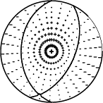
|
|
|
The best fit as a function of depth is given in the following figure:
|
|
|
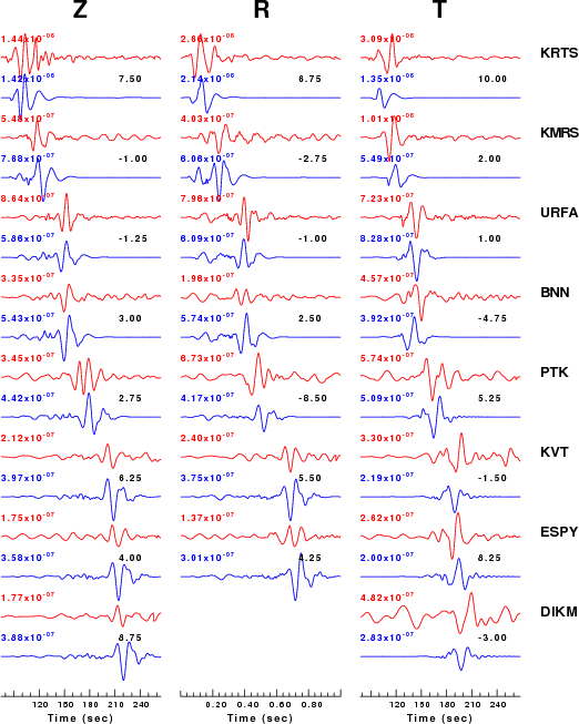
The comparison of the observed and predicted waveforms is given in the next figure. The red traces are the observed and the blue are the predicted. Each observed-predicted componnet is plotted to the same scale and peak amplitudes are indicated by the numbers to the left of each trace. The number in black at the rightr of each predicted traces it the time shift required for maximum correlation between the observed and predicted traces. This time shift is required because the synthetics are not computed at exactly the same distance as the observed and because the velocity model used in the predictions may not be perfect. A positive time shift indicates that the prediction is too fast and should be delayed to match the observed trace (shift to the right in this figure). A negative value indicates that the prediction is too slow. The bandpass filter used in the processing and for the display was
hp c 0.02 n 3
lp c 0.05 n 3
|
|
|
|
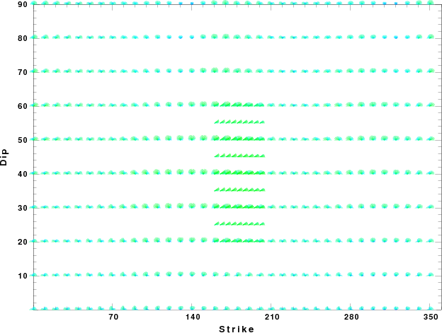
| Focal mechanism sensitivity at the preferred depth. The red color indicates a very good fit to thewavefroms. Each solution is plotted as a vector at a given value of strike and dip with the angle of the vector representing the rake angle, measured, with respect to the upward vertical (N) in the figure. |
The WUS used for the waveform synthetic seismograms and for the surface wave eigenfunctions and dispersion is as follows:
MODEL.01
Model after     8 iterations
ISOTROPIC
KGS
FLAT EARTH
1-D
CONSTANT VELOCITY
LINE08
LINE09
LINE10
LINE11
      H(KM)   VP(KM/S)   VS(KM/S) RHO(GM/CC)         QP         QS       ETAP       ETAS      FREFP      FREFS
     1.9000     3.4065     2.0089     2.2150  0.302E-02  0.679E-02   0.00       0.00       1.00       1.00
     6.1000     5.5445     3.2953     2.6089  0.349E-02  0.784E-02   0.00       0.00       1.00       1.00
    13.0000     6.2708     3.7396     2.7812  0.212E-02  0.476E-02   0.00       0.00       1.00       1.00
    19.0000     6.4075     3.7680     2.8223  0.111E-02  0.249E-02   0.00       0.00       1.00       1.00
     0.0000     7.9000     4.6200     3.2760  0.164E-10  0.370E-10   0.00       0.00       1.00       1.00
Here we tabulate the reasons for not using certain digital data sets
The following stations did not have a valid response files:
DATE=Wed Jun 17 16:02:53 CDT 2009