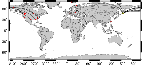
Location of the earthquake (yellow star) and great circle path from the epicenter to each station (red) [created using GMT (Wessel, P., and W. H. F. Smith, New version of Generic Mapping Tools released, EOS Trans. AGU, 76 329, 1995.)]
2007/04/09 10:18:04 48.37 154.65 36
The following compares this source inversion to the USGS Rapid Moment Tensor Solution and to the Harvard CMT solutions, if they are available.
 SLU Moment Tensor Solution
 2007/04/09 10:18:04

 Best Fitting Double Couple
    Mo = 3.63e+24 dyne-cm
    Mw = 5.64
    Z  = 25 km
     Plane   Strike  Dip  Rake
      NP1       44    67   110
      NP2      180    30    50
 Principal Axes:
   Axis    Value   Plunge  Azimuth
     T   3.63e+24     62     346
     N   0.00e+00     19     216
     P  -3.63e+24     20     119


 Moment Tensor: (dyne-cm)
    Component  Value
       Mxx     5.68e+16
       Mxy     1.17e+24
       Mxz     2.02e+24
       Myy    -2.41e+24
       Myz    -1.39e+24
       Mzz     2.41e+24


                     ----##########
                 -----#################
              ------######################
             -----########################-
           ------#########################---
          ------#########################-----
         ------##########   #############------
        ------########### T ############--------
        ------###########   ###########---------
       ------#########################-----------
       ------#######################-------------
       ------######################--------------
       ------####################----------------
        ------#################-----------------
        ------################-----------   ----
         ------############-------------- P ---
          ------#########----------------   --
           ------#####-----------------------
             ------------------------------
              ######----------------------
                 #####-----------------
                     ####----------


 Harvard Convention
 Moment Tensor:
      R          T          F
  2.41e+24   2.02e+24   1.39e+24
  2.02e+24   5.68e+16  -1.17e+24
  1.39e+24  -1.17e+24  -2.41e+24
|
07/04/09 10:18: 4.91
 KURIL ISLANDS
 Epicenter:  48.367  154.653
 MW 5.6

 USGS MOMENT TENSOR SOLUTION
 Depth  33         No. of sta: 70
 Moment Tensor;   Scale 10**17 Nm
   Mrr= 3.63       Mtt=-1.08
   Mpp=-2.55       Mrt= 0.27
   Mrp= 1.29       Mtp=-1.24
  Principal axes:
   T  Val=  3.89  Plg=79  Azm=271
   N       -0.40       5       27
   P       -3.48      10      118

 Best Double Couple:Mo=3.7*10**17
  NP1:Strike=215 Dip=35 Slip=  99
  NP2:        24     55        84

               -------
          ----------------#
        -----------#######---
      ---------############----
    ---------##############------
   --------################-------
   -------#################-------
  -------#################---------
  ------#######   ########---------
  -----######## T #######----------
  -----########   #######----------
  -----#################-----------
   ----################-------   -
   ----###############-------- P -
    ---#############----------
      --###########------------
        ########-------------
          ###--------------
               -------
|
April 9, 2007, KURIL ISLANDS, MW=5.8

Goran Ekstrom

CENTROID-MOMENT-TENSOR  SOLUTION
GCMT EVENT:     C200704091018A
DATA: IU II CU IC
L.P.BODY WAVES: 73S, 165C, T= 40
MANTLE WAVES:   53S,  64C, T=125
SURFACE WAVES:  80S, 175C, T= 50
TIMESTAMP:      Q-20070409141236
CENTROID LOCATION:
ORIGIN TIME:      10:18:07.1 0.1
LAT:48.21N 0.01;LON:155.17E 0.01
DEP: 33.0  0.3;TRIANG HDUR:  1.9
MOMENT TENSOR: SCALE 10**24 D-CM
RR= 4.600 0.058; TT=-1.270 0.041
PP=-3.330 0.044; RT= 1.970 0.066
RP= 2.270 0.063; TP=-2.380 0.032
PRINCIPAL AXES:
1.(T) VAL=  5.486;PLG=73;AZM=318
2.(N)       0.267;     4;    215
3.(P)      -5.753;    16;    124
BEST DBLE.COUPLE:M0= 5.62*10**24
NP1: STRIKE=209;DIP=29;SLIP=  82
NP2: STRIKE= 38;DIP=61;SLIP=  94

            -----------
        --------###########
      -------###############-
    ------##################---
   ------###################----
  ------###################------
  -----#######   ##########------
 -----######## T #########--------
 ----#########   ########---------
 ----###################----------
 ----##################-----------
  ---################------------
  ---###############--------   --
   ---############---------- P -
    --#########-------------
      -#####-----------------
        #------------------
            -----------
|
** These results are from a research system and are not official USGS magnitudes. **

General region :  2007ayaq KURIL ISLANDS
surface waves  (3.0,3.5,7,7.5 mHz)
Stations used : ARU INCN KEV KIP KURK TIXI TLY ULN
Origin time: 2007   99  10  18   4
Original location (lat,lon,depth) :      48.4000    154.700  36
Moment tensor (x1.e26 dyncm) :
Mrr :      0.033683 Mtt :     -0.009472
Mff :     -0.024211 Mrt :      0.036751
Mrf :      0.002139 Mtf :     -0.027409
T-axis:  moment=     0.057   plunge=    56.495  azimuth=    16.566
N-axis:  moment=    -0.004   plunge=    27.429  azimuth=   234.940
P-axis:  moment=    -0.053   plunge=    17.707  azimuth=   135.401
best double couple: Mo=    0.055(x1.e26 dyncm)  Mw=5.8  tau=  2.1
nodal planes (strike/dip/slip):   67.04/ 68.00/119.79     190.24/ 36.42/ 39.11
Centroid location :   48.408   154.977    21.264
Centroid time :      6.608
Variance reduction (%) :  25

                   ***********
               ****--ooooo----****
            *** ---ooo------------***
          **   --ooo-----------------**
         **   --oo--------------------**
        *    --oo-----------------------*
       *     -oo----------T--------------*
      **    -oo------------------------oo**
      *     -o------------------------oo- *
     **     oo----------------------ooo   **
     **     o-----------+--------ooo      **
     **     o-----------------oooo        **
      *     o-------------ooooo           *
      **    oo-------oooooo              **
       *oooooooooooooo                   *
        *    oo                         *
         **   oo                   P  **
          **   oo                    **
            *** oo                ***
               ****oo         ****
                   ***********

          0-   30-  60-  90-  120- 150- 180- 210- 240- 270- 300- 330-
z-comp:     0    0    1    0    0    0    2    2    1    1    0    0
r-comp:     0    0    1    0    0    0    1    1    1    1    0    0
t-comp:     0    0    1    0    0    0    1    1    1    1    0    0
Total number of traces used =  17
number of runs = 9
starttime = Mon Apr 9 04:38:28 MDT 2007
endtime = Mon Apr 9 04:56:31 MDT 2007
inversion time = Mon Apr 9 04:56:28 MDT 2007 - Mon Apr 9 04:56:30 MDT 2007
Solution produced by inversion of all available channels
|
The following broadband stations passed the QC and were used for the source inversion. BFO BLA BMO BRAL COLA EYMN JCT KBS KEV KWP MSO NEW NHSC TATO TPNV
All observed and Greens function waveforms are corrected to instrument response to ground velocity in meters/sec for the passband of 0.004 - 5 Hz. The traces were then lowpass filtered at 0.25 Hz and interpolated to a sample rate of 1 second.
For the grid search, the observed traces and Green's functions are read in an cut using the following commands
Phase    Gsac Command              Comment
 P    cut A -30 A       CUTH = 95+0.3*DEPTH
SH    cut T1 -60 T1     CUTH = 95+0.6*DEPTH
SV    cut T0 -60 T0     CUTH = 95+0.6*DEPTH

where the 95 is a maximum filter duration, DEPTH is in km, and the CUTH in sec
The cut windows attempt to include the P, pP, sP, pS, S and sS arrivals. However, oen must be very careful about the fact that PP may be included in some distance ranges.
The waveforms are then bandpass filtered by the application of the following high- and low-pass stages (an optional microseism filter):
hp c 0.0100 2
lp c 0.0400 2
int
br c 0.12 0.2 n 4 p 2
The traces were next integrated to ground displacment in meters. Finally the observed data are interpolated to ahve the same sampling at the Green's functions.
The source inversion is a multipass operation since a lower frequency filter band is used for larger earthquakes and since a search is made over depth. Up to three passed of the outer loop are made, after which the moment magnitude is determined and filter settings readjusted. The inner loop over depth samples all depths from 0 to 800 km with 5 km increments in depth to 50 km, followed by 10 km depth sampling for the remaining range.
The following filter ranges are used according to the moment magnitude Mw:
   FILTER_BAND   FH(s)  FL(s)
       1           60     12      Mw < 6.4
       2          100     20      6.4 < Mw <= 6.9
       3          120     40      Mw > 6.9
The map displays the distribution of stations used for this source inversion.
|
Location of the earthquake (yellow star) and great circle path from the epicenter to each station (red) [created using GMT (Wessel, P., and W. H. F. Smith, New version of Generic Mapping Tools released, EOS Trans. AGU, 76 329, 1995.)] |
For this data set the favored solution is
WVFMTD96 30.0 39. 62. 81. 5.69 0.581 0.173E-06 0.600 0.763 0.828E-07 27.7
The following figures show the sensitivity of the goodness of fit parameter so source depth, the waveform comparison as a function of epicentral distance in degrees and the source to station azimuth
|
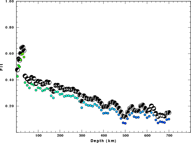
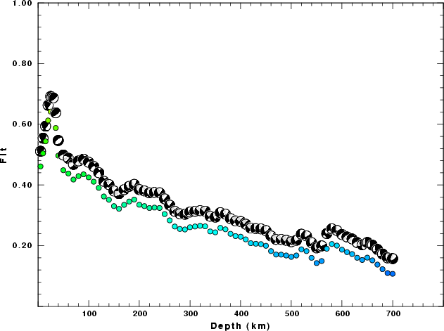
| Goodness of fit as a function of source depth. The measure is 1 - SUM (o -p)2 / SUM o2. A value of 1.0 is the best fit. The best double couple mechanism for the solution depth is plotted above goodness of fit value to indicate how the mefhanism may change with depth. |
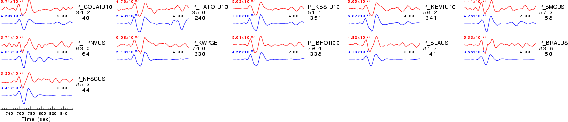
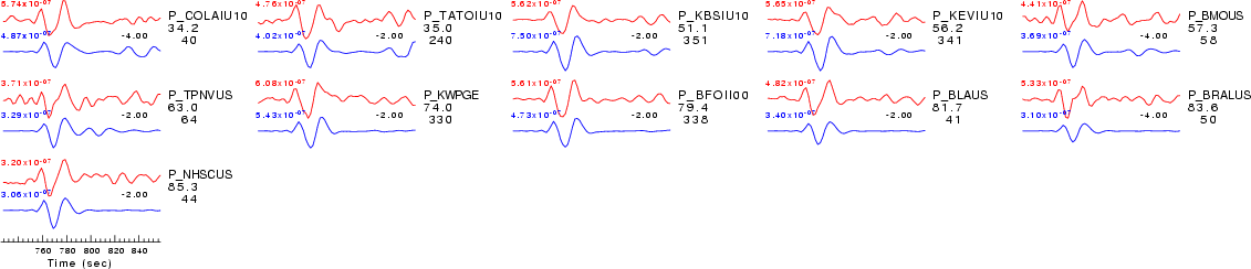
| P-wave Z component |
|
| Comparison of the observed traces (red) and solution predicted traces (blue) ordered in terms of increasing epicentral distance. Each pair of traces is annotated with the station name, epicentral distance in degrees, source to station azimuth in degrees. Each pair of traces is plotted with the same scale and the peak amplitudes are indicated at the lect of each trace. Finally the time shift between the P-wave first arrival picked and the the theoretical P-wave first arrival in the predicted trace is indicated, with a positive sign indicating that the predicted trace has been shifted to the right by the given number of seconds. as a function of source to station azimuth in degrees (D). The purpose of this display is to highlight the azimuthal dependence on the first motion. The traces are annotated with the station name at the top. |
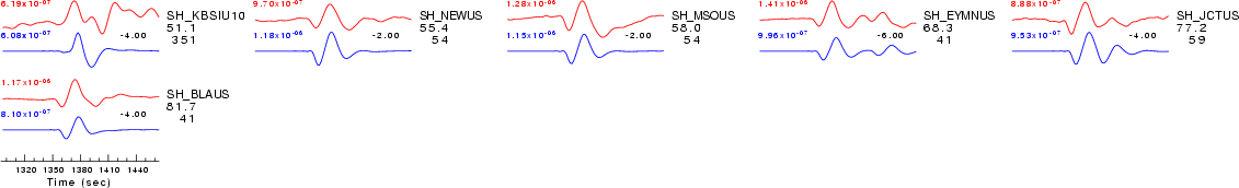
| SH-wave T component |

|
| Comparison of the observed traces (red) and solution predicted traces (blue) ordered in terms of increasing epicentral distance. Each pair of traces is annotated with the station name, epicentral distance in degrees, source to station azimuth in degrees. Each pair of traces is plotted with the same scale and the peak amplitudes are indicated at the lect of each trace. Finally the time shift between the P-wave first arrival picked and the the theoretical P-wave first arrival in the predicted trace is indicated, with a positive sign indicating that the predicted trace has been shifted to the right by the given number of seconds. as a function of source to station azimuth in degrees (D). The purpose of this display is to highlight the azimuthal dependence on the first motion. The traces are annotated with the station name at the top. |
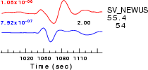
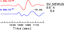
| SV-wave R component |
|
| Comparison of the observed traces (red) and solution predicted traces (blue) ordered in terms of increasing epicentral distance. Each pair of traces is annotated with the station name, epicentral distance in degrees, source to station azimuth in degrees. Each pair of traces is plotted with the same scale and the peak amplitudes are indicated at the lect of each trace. Finally the time shift between the P-wave first arrival picked and the the theoretical P-wave first arrival in the predicted trace is indicated, with a positive sign indicating that the predicted trace has been shifted to the right by the given number of seconds. as a function of source to station azimuth in degrees (D). The purpose of this display is to highlight the azimuthal dependence on the first motion. The traces are annotated with the station name at the top. |
All observed and Greens function waveforms are corrected to instrument response to ground velocity in meters/sec for the passband of 0.004 - 5 Hz. The traces were then lowpass filtered at 0.25 Hz and interpolated to a sample rate of 1 second.
For the grid search, the observed traces and Green's functions are read in an cut using the following commands
Phase    Gsac Command              Comment
 P    cut A -30 A       CUTH = 95+0.3*DEPTH
SH    cut T1 -60 T1     CUTH = 95+0.6*DEPTH
SV    cut T0 -60 T0     CUTH = 95+0.6*DEPTH

where the 95 is a maximum filter duration, DEPTH is in km, and the CUTH in sec
The cut windows attempt to include the P, pP, sP, pS, S and sS arrivals. However, oen must be very careful about the fact that PP may be included in some distance ranges.
The waveforms are then bandpass filtered by the application of the following high- and low-pass stages (an optional microseism filter):
hp c 0.0100 2
lp c 0.0400 2
int
br c 0.12 0.2 n 4 p 2
The traces were next integrated to ground displacment in meters. Finally the observed data are interpolated to ahve the same sampling at the Green's functions.
The source inversion is a multipass operation since a lower frequency filter band is used for larger earthquakes and since a search is made over depth. Up to three passed of the outer loop are made, after which the moment magnitude is determined and filter settings readjusted. The inner loop over depth samples all depths from 0 to 800 km with 5 km increments in depth to 50 km, followed by 10 km depth sampling for the remaining range.
The following filter ranges are used according to the moment magnitude Mw:
   FILTER_BAND   FH(s)  FL(s)
       1           60     12      Mw < 6.4
       2          100     20      6.4 < Mw <= 6.9
       3          120     40      Mw > 6.9
The map displays the distribution of stations used for this source inversion.

Location of the earthquake (yellow star) and great circle path from the epicenter to each station (red) [created using GMT (Wessel, P., and W. H. F. Smith, New version of Generic Mapping Tools released, EOS Trans. AGU, 76 329, 1995.)] |
For this data set the favored solution is
WVFGRD96 25.0 180 30 50 5.64 0.6417
The following figures show the sensitivity of the goodness of fit parameter so source depth, the waveform comparison as a function of epicentral distance in degrees and the source to station azimuth
|
| Goodness of fit as a function of source depth. The measure is 1 - SUM (o -p)2 / SUM o2. A value of 1.0 is the best fit. The best double couple mechanism for the solution depth is plotted above goodness of fit value to indicate how the mefhanism may change with depth. |
| P-wave Z component |
|
| Comparison of the observed traces (red) and solution predicted traces (blue) ordered in terms of increasing epicentral distance. Each pair of traces is annotated with the station name, epicentral distance in degrees, source to station azimuth in degrees. Each pair of traces is plotted with the same scale and the peak amplitudes are indicated at the lect of each trace. Finally the time shift between the P-wave first arrival picked and the the theoretical P-wave first arrival in the predicted trace is indicated, with a positive sign indicating that the predicted trace has been shifted to the right by the given number of seconds. as a function of source to station azimuth in degrees (D). The purpose of this display is to highlight the azimuthal dependence on the first motion. The traces are annotated with the station name at the top. |
| SH-wave T component |
|
| Comparison of the observed traces (red) and solution predicted traces (blue) ordered in terms of increasing epicentral distance. Each pair of traces is annotated with the station name, epicentral distance in degrees, source to station azimuth in degrees. Each pair of traces is plotted with the same scale and the peak amplitudes are indicated at the lect of each trace. Finally the time shift between the P-wave first arrival picked and the the theoretical P-wave first arrival in the predicted trace is indicated, with a positive sign indicating that the predicted trace has been shifted to the right by the given number of seconds. as a function of source to station azimuth in degrees (D). The purpose of this display is to highlight the azimuthal dependence on the first motion. The traces are annotated with the station name at the top. |
| SV-wave R component |
|
| Comparison of the observed traces (red) and solution predicted traces (blue) ordered in terms of increasing epicentral distance. Each pair of traces is annotated with the station name, epicentral distance in degrees, source to station azimuth in degrees. Each pair of traces is plotted with the same scale and the peak amplitudes are indicated at the lect of each trace. Finally the time shift between the P-wave first arrival picked and the the theoretical P-wave first arrival in the predicted trace is indicated, with a positive sign indicating that the predicted trace has been shifted to the right by the given number of seconds. as a function of source to station azimuth in degrees (D). The purpose of this display is to highlight the azimuthal dependence on the first motion. The traces are annotated with the station name at the top. |