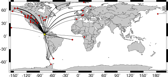
Location of the earthquake (yellow star) and great circle path from the epicenter to each station (red) [created using GMT (Wessel, P., and W. H. F. Smith, New version of Generic Mapping Tools released, EOS Trans. AGU, 76 329, 1995.)]
2007/03/18 02:11:05 4.55 -78.50 10
The following compares this source inversion to the USGS Rapid Moment Tensor Solution and to the Harvard CMT solutions, if they are available.
 SLU Moment Tensor Solution
 2007/03/18 02:11:05

 Best Fitting Double Couple
    Mo = 1.78e+25 dyne-cm
    Mw = 6.10
    Z  = 5 km
     Plane   Strike  Dip  Rake
      NP1       70    75   -55
      NP2      180    38   -155
 Principal Axes:
   Axis    Value   Plunge  Azimuth
     T   1.78e+25     22     134
     N   0.00e+00     34     240
     P  -1.78e+25     48      17


 Moment Tensor: (dyne-cm)
    Component  Value
       Mxx     9.85e+22
       Mxy    -9.89e+24
       Mxz    -1.28e+25
       Myy     7.18e+24
       Myz     1.83e+24
       Mzz    -7.28e+24


                     ####----------
                 ######----------------
              #######---------------------
             ######------------------------
           #######------------   ------------
          #######------------- P -------------
         #######--------------   --------------
        ########-------------------------------#
        #######------------------------------###
       ########---------------------------#######
       ########------------------------##########
       ########---------------------#############
       ########----------------##################
        #######-----------######################
        ########---#############################
         -------###############################
          -------#####################   #####
           -------#################### T ####
             ------###################   ##
              -------#####################
                 ------################
                     ----##########


 Harvard Convention
 Moment Tensor:
      R          T          F
 -7.28e+24  -1.28e+25  -1.83e+24
 -1.28e+25   9.85e+22   9.89e+24
 -1.83e+24   9.89e+24   7.18e+24
|
07/03/18 02:11: 5.91
 SOUTH OF PANAMA
 Epicenter:   4.576  -78.490
 MW 6.1

 USGS MOMENT TENSOR SOLUTION
 Depth   7         No. of sta: 71
 Moment Tensor;   Scale 10**18 Nm
   Mrr=-1.48       Mtt= 0.83
   Mpp= 0.65       Mrt=-0.92
   Mrp= 0.47       Mtp= 1.28
  Principal axes:
   T  Val=  2.06  Plg= 6  Azm=139
   N        0.05      31      233
   P       -2.11      58       39

 Best Double Couple:Mo=2.1*10**18
  NP1:Strike=199 Dip=47 Slip=-135
  NP2:        75     59       -53

               #######
          ###########------
        ##########-----------
      ##########---------------
    ##########-------------------
   ##########--------   ----------
   #########--------- P ----------
  #########----------   ----------#
  #########----------------------##
  ########---------------------####
  ########-------------------######
  ########---------------##########
   --#####-----------#############
   -------########################
    ------#################   ###
      ----################# T #
        ---################
          --###############
               #######
|
March 18, 2007, SOUTH OF PANAMA, MW=6.2

Meredith Nettles

CENTROID-MOMENT-TENSOR  SOLUTION
GCMT EVENT:     C200703180211A
DATA: IU II IC CU
L.P.BODY WAVES: 72S, 158C, T= 40
MANTLE WAVES:   73S, 118C, T=125
SURFACE WAVES:  79S, 193C, T= 50
TIMESTAMP:      Q-20070318112332
CENTROID LOCATION:
ORIGIN TIME:      02:11:11.2 0.1
LAT: 4.71N 0.00;LON: 78.53W 0.00
DEP: 12.0  FIX;TRIANG HDUR:  3.1
MOMENT TENSOR: SCALE 10**25 D-CM
RR=-2.390 0.012; TT= 0.339 0.011
PP= 2.050 0.014; RT=-0.037 0.033
RP= 1.170 0.036; TP= 0.901 0.010
PRINCIPAL AXES:
1.(T) VAL=  2.664;PLG=12;AZM=291
2.(N)       0.037;    10;    199
3.(P)      -2.701;    74;     71
BEST DBLE.COUPLE:M0= 2.68*10**25
NP1: STRIKE= 34;DIP=34;SLIP= -72
NP2: STRIKE=193;DIP=58;SLIP=-101

            ########---
        ##########---------
      ##########------------#
    ###########--------------##
   ###########---------------###
     ########-----------------###
   T #######------------------###
 #   #######-------   --------####
 ##########-------- P -------#####
 ##########--------   -------#####
 ##########-----------------######
  ########------------------#####
  #########---------------#######
   ########--------------#######
    #######------------########
      ######--------#########
        ####----###########
            -##########
|
The following broadband stations passed the QC and were used for the source inversion. AAM ADK AHID ASCN BFO BLA BMO BW06 CBKS CBN COLA COR EFI EGAK EGMT EYMN GRFO HKT KBS KDAK KEV KONO LONY MNTX MSKU NATX NEW NLWA PAB PMSA POHA TUC WMOK WRAK WUAZ WVOR
All observed and Greens function waveforms are corrected to instrument response to ground velocity in meters/sec for the passband of 0.004 - 5 Hz. The traces were then lowpass filtered at 0.25 Hz and interpolated to a sample rate of 1 second.
For the grid search, the observed traces and Green's functions are read in an cut using the following commands
Phase    Gsac Command              Comment
 P    cut A -30 A       CUTH = 95+0.3*DEPTH
SH    cut T1 -60 T1     CUTH = 95+0.6*DEPTH
SV    cut T0 -60 T0     CUTH = 95+0.6*DEPTH

where the 95 is a maximum filter duration, DEPTH is in km, and the CUTH in sec
The cut windows attempt to include the P, pP, sP, pS, S and sS arrivals. However, oen must be very careful about the fact that PP may be included in some distance ranges.
The waveforms are then bandpass filtered by the application of the following high- and low-pass stages (an optional microseism filter):
hp c 0.0100 2
lp c 0.0400 2
int
br c 0.12 0.2 n 4 p 2
The traces were next integrated to ground displacment in meters. Finally the observed data are interpolated to ahve the same sampling at the Green's functions.
The source inversion is a multipass operation since a lower frequency filter band is used for larger earthquakes and since a search is made over depth. Up to three passed of the outer loop are made, after which the moment magnitude is determined and filter settings readjusted. The inner loop over depth samples all depths from 0 to 800 km with 5 km increments in depth to 50 km, followed by 10 km depth sampling for the remaining range.
The following filter ranges are used according to the moment magnitude Mw:
   FILTER_BAND   FH(s)  FL(s)
       1           60     12      Mw < 6.4
       2          100     20      6.4 < Mw <= 6.9
       3          120     40      Mw > 6.9
The map displays the distribution of stations used for this source inversion.
|
Location of the earthquake (yellow star) and great circle path from the epicenter to each station (red) [created using GMT (Wessel, P., and W. H. F. Smith, New version of Generic Mapping Tools released, EOS Trans. AGU, 76 329, 1995.)] |
For this data set the favored solution is
WVFGRD96 5.0 70 75 -55 6.10 0.5472
The following figures show the sensitivity of the goodness of fit parameter so source depth, the waveform comparison as a function of epicentral distance in degrees and the source to station azimuth
|
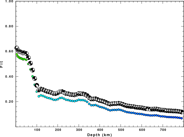
| Goodness of fit as a function of source depth. The measure is 1 - SUM (o -p)2 / SUM o2. A value of 1.0 is the best fit. The best double couple mechanism for the solution depth is plotted above goodness of fit value to indicate how the mefhanism may change with depth. |
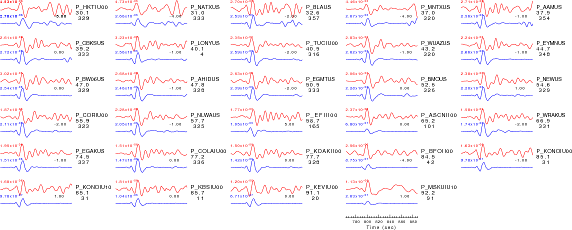
| P-wave Z component |
|
| Comparison of the observed traces (red) and solution predicted traces (blue) ordered in terms of increasing epicentral distance. Each pair of traces is annotated with the station name, epicentral distance in degrees, source to station azimuth in degrees. Each pair of traces is plotted with the same scale and the peak amplitudes are indicated at the lect of each trace. Finally the time shift between the P-wave first arrival picked and the the theoretical P-wave first arrival in the predicted trace is indicated, with a positive sign indicating that the predicted trace has been shifted to the right by the given number of seconds. as a function of source to station azimuth in degrees (D). The purpose of this display is to highlight the azimuthal dependence on the first motion. The traces are annotated with the station name at the top. |
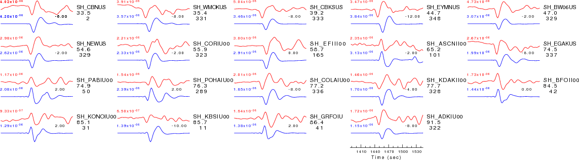
| SH-wave T component |
|
| Comparison of the observed traces (red) and solution predicted traces (blue) ordered in terms of increasing epicentral distance. Each pair of traces is annotated with the station name, epicentral distance in degrees, source to station azimuth in degrees. Each pair of traces is plotted with the same scale and the peak amplitudes are indicated at the lect of each trace. Finally the time shift between the P-wave first arrival picked and the the theoretical P-wave first arrival in the predicted trace is indicated, with a positive sign indicating that the predicted trace has been shifted to the right by the given number of seconds. as a function of source to station azimuth in degrees (D). The purpose of this display is to highlight the azimuthal dependence on the first motion. The traces are annotated with the station name at the top. |
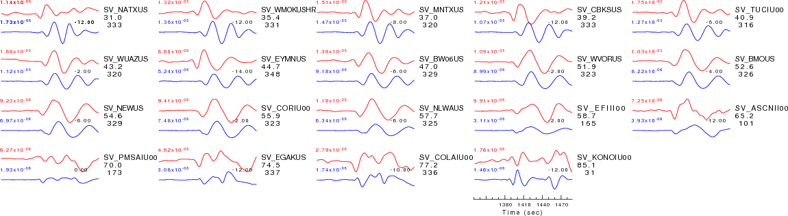
| SV-wave R component |
|
| Comparison of the observed traces (red) and solution predicted traces (blue) ordered in terms of increasing epicentral distance. Each pair of traces is annotated with the station name, epicentral distance in degrees, source to station azimuth in degrees. Each pair of traces is plotted with the same scale and the peak amplitudes are indicated at the lect of each trace. Finally the time shift between the P-wave first arrival picked and the the theoretical P-wave first arrival in the predicted trace is indicated, with a positive sign indicating that the predicted trace has been shifted to the right by the given number of seconds. as a function of source to station azimuth in degrees (D). The purpose of this display is to highlight the azimuthal dependence on the first motion. The traces are annotated with the station name at the top. |