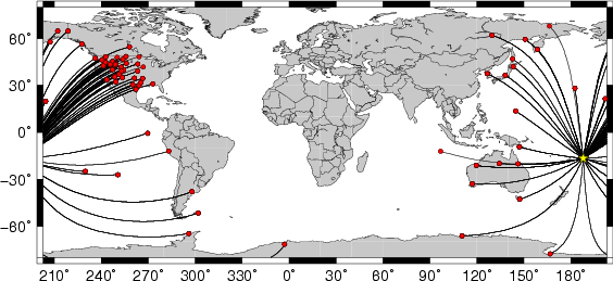
Location of the earthquake (yellow star) and great circle path from the epicenter to each station (red) [created using GMT (Wessel, P., and W. H. F. Smith, New version of Generic Mapping Tools released, EOS Trans. AGU, 76 329, 1995.)]
2006/09/28 06:22:09 -16.59 -172.03 28
The following compares this source inversion to the USGS Rapid Moment Tensor Solution and to the Harvard CMT solutions, if they are available.
 SLU Moment Tensor Solution
 2006/09/28 06:22:09

 Best Fitting Double Couple
    Mo = 1.11e+26 dyne-cm
    Mw = 6.63
    Z  = 5 km
     Plane   Strike  Dip  Rake
      NP1      175    53   -106
      NP2       20    40   -70
 Principal Axes:
   Axis    Value   Plunge  Azimuth
     T   1.11e+26      7     276
     N   0.00e+00     13     184
     P  -1.11e+26     76      33


 Moment Tensor: (dyne-cm)
    Component  Value
       Mxx    -3.67e+24
       Mxy    -1.43e+25
       Mxz    -2.11e+25
       Myy     1.06e+26
       Myz    -2.69e+25
       Mzz    -1.03e+26


                     ####----------
                 ######--------------##
              ########----------------####
             ########------------------####
           #########--------------------#####
          ##########---------------------#####
         ##########----------------------######
        ###########----------------------#######
          #########---------   ----------#######
        T #########--------- P ----------########
          #########---------   ----------########
       ############----------------------########
       ############---------------------#########
        ###########---------------------########
        ############-------------------#########
         ###########------------------#########
          ###########----------------#########
           ###########-------------##########
             ##########----------##########
              ##########-------###########
                 #########--###########
                     #------#######


 Harvard Convention
 Moment Tensor:
      R          T          F
 -1.03e+26  -2.11e+25   2.69e+25
 -2.11e+25  -3.67e+24   1.43e+25
  2.69e+25   1.43e+25   1.06e+26
|
The following broadband stations passed the QC and were used for the source inversion. AGMN ANMO BILL BMO BRAL CASY COCO COLA CTAO DGMT DLMT DUG ECSD EFI EGAK EGMT ERM FFC FLWY GUMO HAWA HKT HLID IMW INCN ISCO JCT KDAK KIP KSU1 KVTX LAO LOHW MA2 MAJO MBWA MIAR MIDW MOOW MVCO NATX NEW NLWA NNA NWAO PAYG PET PFO PMG PMSA POHA PTCN REDW RPN RRI2 RSSD RWWY SBA SCIA SMCO SNAA SNOW TAU TPAW TRQA TUC WMOK WRAB WRAK WUAZ WVOR YAK YSS
All observed and Greens function waveforms are corrected to instrument response to ground velocity in meters/sec for the passband of 0.004 - 5 Hz. The traces were then lowpass filtered at 0.25 Hz and interpolated to a sample rate of 1 second.
For the grid search, the observed traces and Green's functions are read in an cut using the following commands
Phase    Gsac Command              Comment
 P    cut A -30 A       CUTH = 95+0.3*DEPTH
SH    cut T1 -60 T1     CUTH = 95+0.6*DEPTH
SV    cut T0 -60 T0     CUTH = 95+0.6*DEPTH

where the 95 is a maximum filter duration, DEPTH is in km, and the CUTH in sec
The cut windows attempt to include the P, pP, sP, pS, S and sS arrivals. However, oen must be very careful about the fact that PP may be included in some distance ranges.
The waveforms are then bandpass filtered by the application of the following high- and low-pass stages (an optional microseism filter):
hp c 0.0100 2
lp c 0.0400 2
int
br c 0.12 0.2 n 4 p 2
The traces were next integrated to ground displacment in meters. Finally the observed data are interpolated to ahve the same sampling at the Green's functions.
The source inversion is a multipass operation since a lower frequency filter band is used for larger earthquakes and since a search is made over depth. Up to three passed of the outer loop are made, after which the moment magnitude is determined and filter settings readjusted. The inner loop over depth samples all depths from 0 to 800 km with 5 km increments in depth to 50 km, followed by 10 km depth sampling for the remaining range.
The following filter ranges are used according to the moment magnitude Mw:
   FILTER_BAND   FH(s)  FL(s)
       1           60     12      Mw < 6.4
       2          100     20      6.4 < Mw <= 6.9
       3          120     40      Mw > 6.9
The map displays the distribution of stations used for this source inversion.
|
Location of the earthquake (yellow star) and great circle path from the epicenter to each station (red) [created using GMT (Wessel, P., and W. H. F. Smith, New version of Generic Mapping Tools released, EOS Trans. AGU, 76 329, 1995.)] |
For this data set the favored solution is
WVFMTD96 40.0 195. 67. -67. 6.73 0.342 0.952E-05 0.355 0.586 0.431E-05 39.8
The following figures show the sensitivity of the goodness of fit parameter so source depth, the waveform comparison as a function of epicentral distance in degrees and the source to station azimuth
|
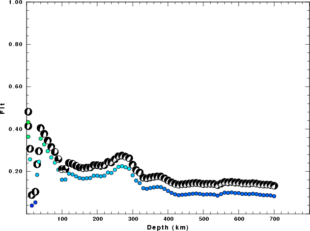
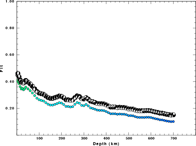
| Goodness of fit as a function of source depth. The measure is 1 - SUM (o -p)2 / SUM o2. A value of 1.0 is the best fit. The best double couple mechanism for the solution depth is plotted above goodness of fit value to indicate how the mefhanism may change with depth. |
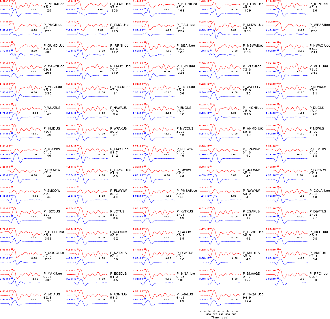
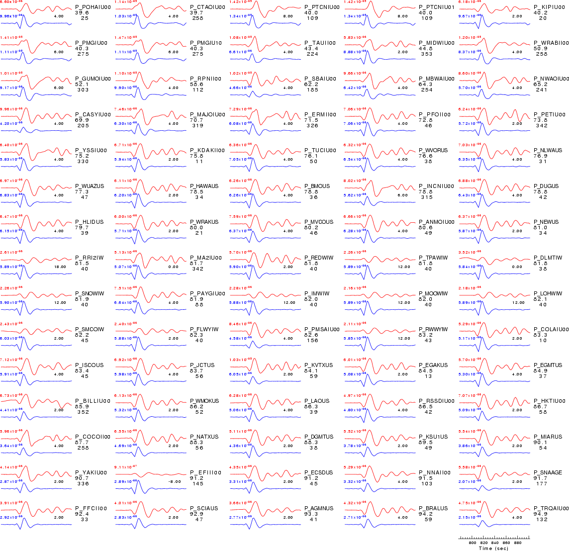
| P-wave Z component |
|
| Comparison of the observed traces (red) and solution predicted traces (blue) ordered in terms of increasing epicentral distance. Each pair of traces is annotated with the station name, epicentral distance in degrees, source to station azimuth in degrees. Each pair of traces is plotted with the same scale and the peak amplitudes are indicated at the lect of each trace. Finally the time shift between the P-wave first arrival picked and the the theoretical P-wave first arrival in the predicted trace is indicated, with a positive sign indicating that the predicted trace has been shifted to the right by the given number of seconds. as a function of source to station azimuth in degrees (D). The purpose of this display is to highlight the azimuthal dependence on the first motion. The traces are annotated with the station name at the top. |
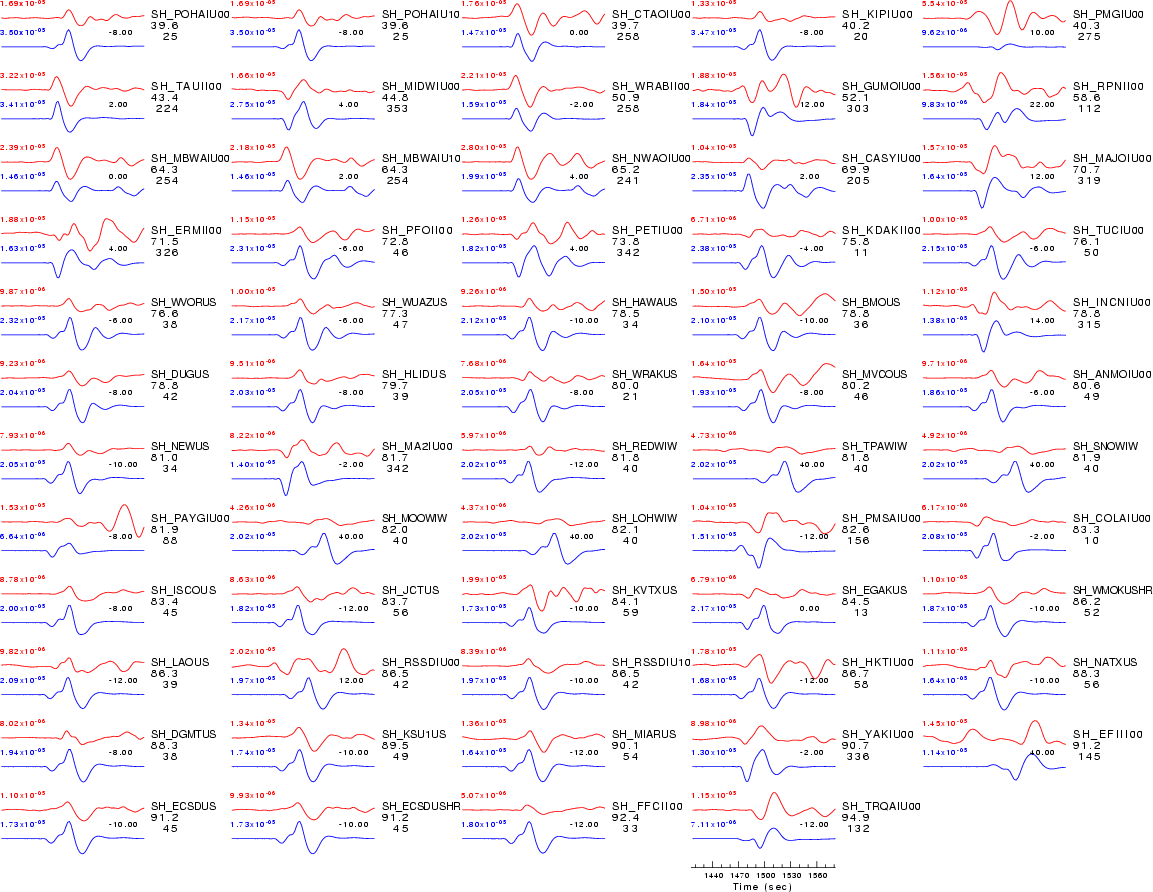
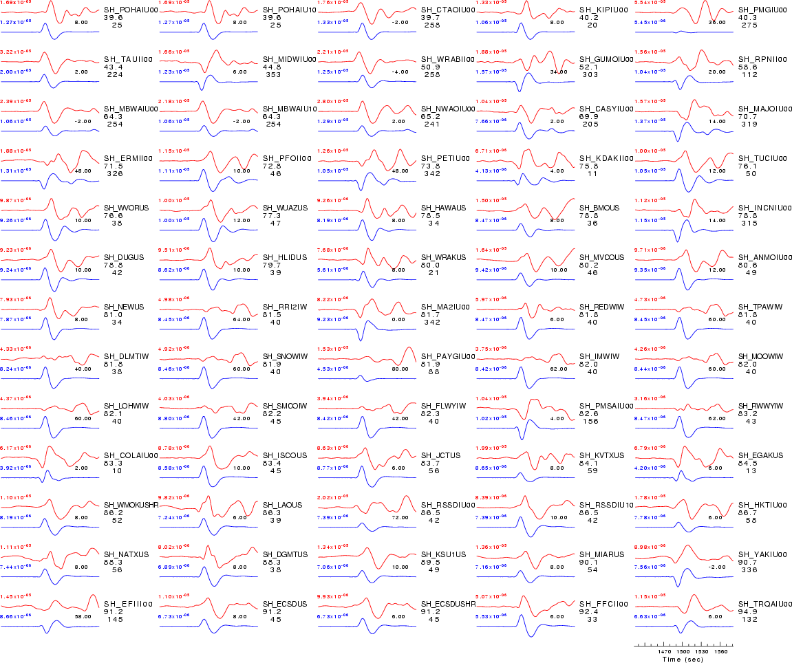
| SH-wave T component |
|
| Comparison of the observed traces (red) and solution predicted traces (blue) ordered in terms of increasing epicentral distance. Each pair of traces is annotated with the station name, epicentral distance in degrees, source to station azimuth in degrees. Each pair of traces is plotted with the same scale and the peak amplitudes are indicated at the lect of each trace. Finally the time shift between the P-wave first arrival picked and the the theoretical P-wave first arrival in the predicted trace is indicated, with a positive sign indicating that the predicted trace has been shifted to the right by the given number of seconds. as a function of source to station azimuth in degrees (D). The purpose of this display is to highlight the azimuthal dependence on the first motion. The traces are annotated with the station name at the top. |
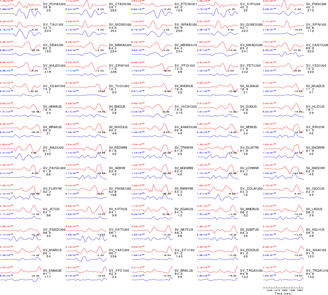
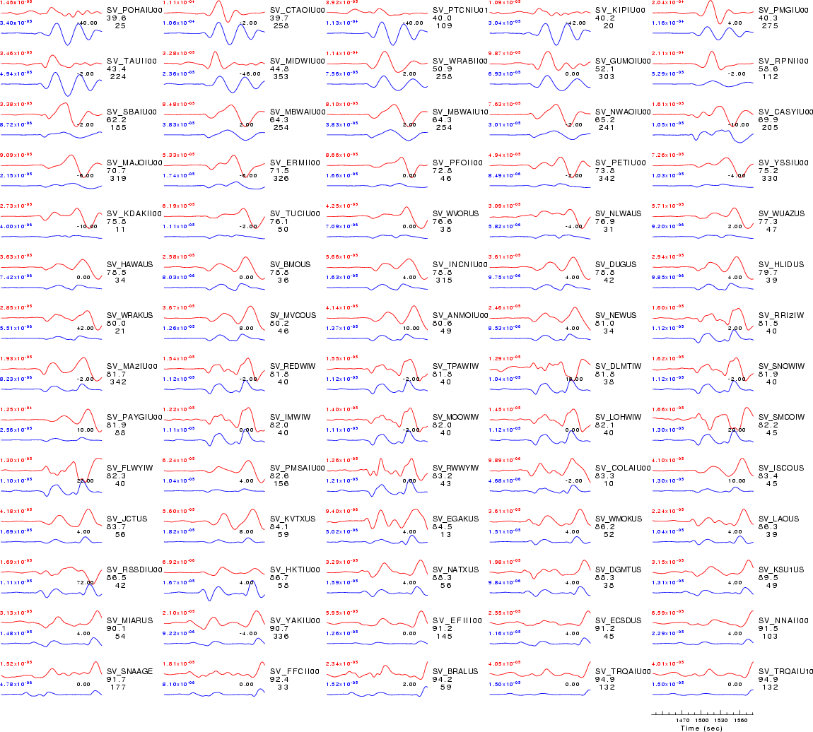
| SV-wave R component |
|
| Comparison of the observed traces (red) and solution predicted traces (blue) ordered in terms of increasing epicentral distance. Each pair of traces is annotated with the station name, epicentral distance in degrees, source to station azimuth in degrees. Each pair of traces is plotted with the same scale and the peak amplitudes are indicated at the lect of each trace. Finally the time shift between the P-wave first arrival picked and the the theoretical P-wave first arrival in the predicted trace is indicated, with a positive sign indicating that the predicted trace has been shifted to the right by the given number of seconds. as a function of source to station azimuth in degrees (D). The purpose of this display is to highlight the azimuthal dependence on the first motion. The traces are annotated with the station name at the top. |
All observed and Greens function waveforms are corrected to instrument response to ground velocity in meters/sec for the passband of 0.004 - 5 Hz. The traces were then lowpass filtered at 0.25 Hz and interpolated to a sample rate of 1 second.
For the grid search, the observed traces and Green's functions are read in an cut using the following commands
Phase    Gsac Command              Comment
 P    cut A -30 A       CUTH = 95+0.3*DEPTH
SH    cut T1 -60 T1     CUTH = 95+0.6*DEPTH
SV    cut T0 -60 T0     CUTH = 95+0.6*DEPTH

where the 95 is a maximum filter duration, DEPTH is in km, and the CUTH in sec
The cut windows attempt to include the P, pP, sP, pS, S and sS arrivals. However, oen must be very careful about the fact that PP may be included in some distance ranges.
The waveforms are then bandpass filtered by the application of the following high- and low-pass stages (an optional microseism filter):
hp c 0.0100 2
lp c 0.0400 2
int
br c 0.12 0.2 n 4 p 2
The traces were next integrated to ground displacment in meters. Finally the observed data are interpolated to ahve the same sampling at the Green's functions.
The source inversion is a multipass operation since a lower frequency filter band is used for larger earthquakes and since a search is made over depth. Up to three passed of the outer loop are made, after which the moment magnitude is determined and filter settings readjusted. The inner loop over depth samples all depths from 0 to 800 km with 5 km increments in depth to 50 km, followed by 10 km depth sampling for the remaining range.
The following filter ranges are used according to the moment magnitude Mw:
   FILTER_BAND   FH(s)  FL(s)
       1           60     12      Mw < 6.4
       2          100     20      6.4 < Mw <= 6.9
       3          120     40      Mw > 6.9
The map displays the distribution of stations used for this source inversion.

Location of the earthquake (yellow star) and great circle path from the epicenter to each station (red) [created using GMT (Wessel, P., and W. H. F. Smith, New version of Generic Mapping Tools released, EOS Trans. AGU, 76 329, 1995.)] |
For this data set the favored solution is
WVFGRD96 5.0 20 40 -70 6.63 0.4100
The following figures show the sensitivity of the goodness of fit parameter so source depth, the waveform comparison as a function of epicentral distance in degrees and the source to station azimuth
|
| Goodness of fit as a function of source depth. The measure is 1 - SUM (o -p)2 / SUM o2. A value of 1.0 is the best fit. The best double couple mechanism for the solution depth is plotted above goodness of fit value to indicate how the mefhanism may change with depth. |
| P-wave Z component |
|
| Comparison of the observed traces (red) and solution predicted traces (blue) ordered in terms of increasing epicentral distance. Each pair of traces is annotated with the station name, epicentral distance in degrees, source to station azimuth in degrees. Each pair of traces is plotted with the same scale and the peak amplitudes are indicated at the lect of each trace. Finally the time shift between the P-wave first arrival picked and the the theoretical P-wave first arrival in the predicted trace is indicated, with a positive sign indicating that the predicted trace has been shifted to the right by the given number of seconds. as a function of source to station azimuth in degrees (D). The purpose of this display is to highlight the azimuthal dependence on the first motion. The traces are annotated with the station name at the top. |
| SH-wave T component |
|
| Comparison of the observed traces (red) and solution predicted traces (blue) ordered in terms of increasing epicentral distance. Each pair of traces is annotated with the station name, epicentral distance in degrees, source to station azimuth in degrees. Each pair of traces is plotted with the same scale and the peak amplitudes are indicated at the lect of each trace. Finally the time shift between the P-wave first arrival picked and the the theoretical P-wave first arrival in the predicted trace is indicated, with a positive sign indicating that the predicted trace has been shifted to the right by the given number of seconds. as a function of source to station azimuth in degrees (D). The purpose of this display is to highlight the azimuthal dependence on the first motion. The traces are annotated with the station name at the top. |
| SV-wave R component |
|
| Comparison of the observed traces (red) and solution predicted traces (blue) ordered in terms of increasing epicentral distance. Each pair of traces is annotated with the station name, epicentral distance in degrees, source to station azimuth in degrees. Each pair of traces is plotted with the same scale and the peak amplitudes are indicated at the lect of each trace. Finally the time shift between the P-wave first arrival picked and the the theoretical P-wave first arrival in the predicted trace is indicated, with a positive sign indicating that the predicted trace has been shifted to the right by the given number of seconds. as a function of source to station azimuth in degrees (D). The purpose of this display is to highlight the azimuthal dependence on the first motion. The traces are annotated with the station name at the top. |
Starting Processing         : Sat Apr 14 19:41:06 UTC 2007
Starting query to get files : Sat Apr 14 19:41:06 UTC 2007
Starting stareq for response: Sat Apr 14 19:42:55 UTC 2007
Starting deconvolution      : Sat Apr 14 19:45:13 UTC 2007
Starting trace rotation     : Sat Apr 14 19:46:10 UTC 2007
Starting distance selection : Sat Apr 14 19:46:27 UTC 2007
Starting trace QC           : Sat Apr 14 19:46:32 UTC 2007
Starting MTD                : Sat Apr 14 19:58:40 UTC 2007
Starting Grid Search        : Sat Apr 14 20:17:55 UTC 2007
Starting documentation      : Sat Apr 14 20:47:49 UTC 2007
Processing Completion       : Sat Apr 14 20:47:50 UTC 2007