Iran

Location

2006/06/29 21:02:09 55.84N 26.97E 10 5.7 Iran

Arrival Times (from USGS)

Felt Map

Focal Mechanism

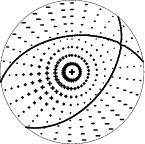
SLU Moment Tensor Solution 2006/06/29 21:02:09 55.84N 26.97E 10 5.7 Iran Best Fitting Double Couple Mo = 5.82e+24 dyne-cm Mw = 5.81 Z = 9 km Plane Strike Dip Rake NP1 40 50 60 NP2 262 48 121 Principal Axes: Axis Value Plunge Azimuth T 5.82e+24 67 243 N 0.00e+00 23 60 P -5.82e+24 1 151 Moment Tensor: (dyne-cm) Component Value Mxx -4.25e+24 Mxy 2.83e+24 Mxz -8.70e+23 Myy -7.18e+23 Myz -1.87e+24 Mzz 4.96e+24 -------------- ---------------------- ---------------------------# -----------------------------# -------------------------------### ----------------##########------#### ----------############################ --------##########################---### -----#############################-----# ----##############################-------- ---##############################--------- -############# ###############---------- ############## T ##############----------- ############# #############----------- ############################------------ #########################------------- ######################-------------- ###################--------------- #############----------------- #######---------------- -- -------------------- P -------------- Harvard Convention Moment Tensor: R T F 4.96e+24 -8.70e+23 1.87e+24 -8.70e+23 -4.25e+24 -2.83e+24 1.87e+24 -2.83e+24 -7.18e+23 Details of the solution is found at http://www.eas.slu.edu/Earthquake_Center/NEW/20060628210209/index.html

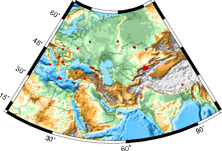
The focal mechanism was determined using broadband seismic waveforms. The location of the event and the station distribution are given in Figure 1.

Figure 1. Location of broadband stations used to obtain focal mechanism

Preferred Solution

The preferred solution from an analysis of the surface-wave spectral amplitude radiation pattern, waveform inversion and first motion observations is

      STK = 40
      DIP = 50
     RAKE = 60
       MW = 5.81
       HS = 9

The solution given here is from the surface--wave spectral amplitude technique.

First motion data

The P-wave first motion data for focal mechanism studies are as follow:

Sta Az(deg)    Dist(km)   First motion
GNI       328 1785 iP_C
MALT      312 2056 iP_C
KSDI      294 2059 iP_D
CSS       298 2319 iP_C

Quality control

The following stations were not used because of excessive low frequency noise in the deconvolved waveforms:

Surface-Wave Focal Mechanism


  NODAL PLANES 

  
  STK=      40.00
  DIP=      50.00
 RAKE=      59.99
  
             OR
  
  STK=     261.93
  DIP=      48.45
 RAKE=     120.79
 
 
DEPTH = 9.0 km
 
Mw = 5.81
Best Fit 0.8522 - P-T axis plot gives solutions with FIT greater than FIT90

First motion data

The P-wave first motion data for focal mechanism studies are as follow:

Sta Az(deg)    Dist(km)   First motion
GNI       328 1785 iP_C
MALT      312 2056 iP_C
KSDI      294 2059 iP_D
CSS       298 2319 iP_C

Surface-wave analysis

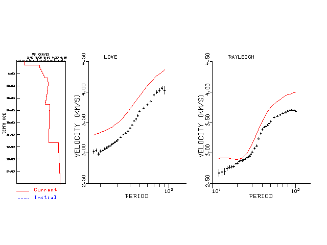
Surface wave analysis was performed using codes from Computer Programs in Seismology, specifically the multiple filter analysis program do_mft and the surface-wave radiation pattern search program srfgrd96.

The velocity model used for the search is a modified Utah model .

Data preparation

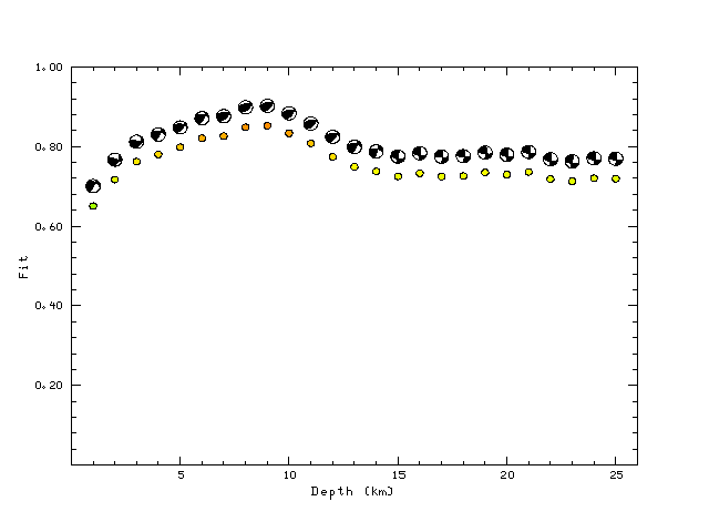
Digital data were collected, instrument response removed and traces converted to Z, R an T components. Multiple filter analysis was applied to the Z and T traces to obtain the Rayleigh- and Love-wave spectral amplitudes, respectively. These were input to the search program which examined all depths between 1 and 25 km and all possible mechanisms.

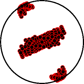
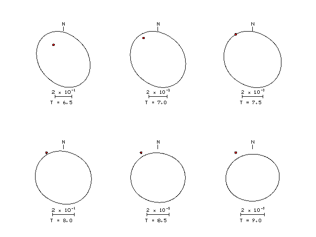
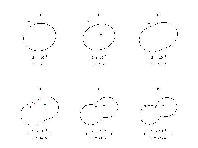
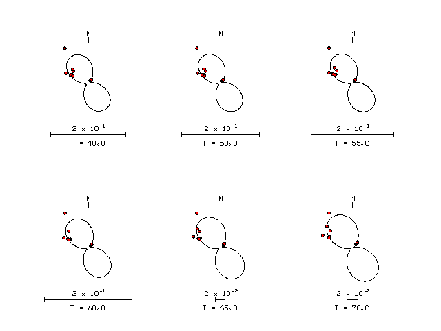
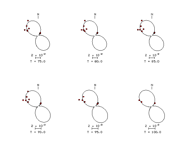
Best mechanism fit as a function of depth. The preferred depth is given above. Lower hemisphere projection

Pressure-tension axis trends. Since the surface-wave spectra search does not distinguish between P and T axes and since there is a 180 ambiguity in strike, all possible P and T axes are plotted. First motion data and waveforms will be used to select the preferred mechanism. The purpose of this plot is to provide an idea of the possible range of solutions. The P and T-axes for all mechanisms with goodness of fit greater than 0.9 FITMAX (above) are plotted here.

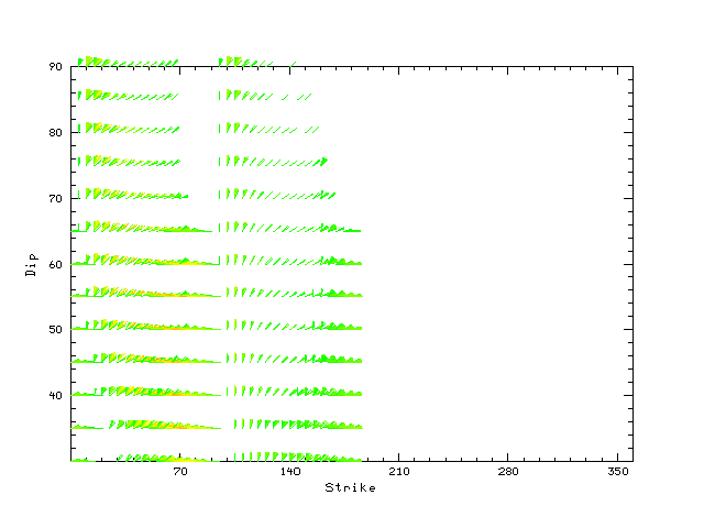
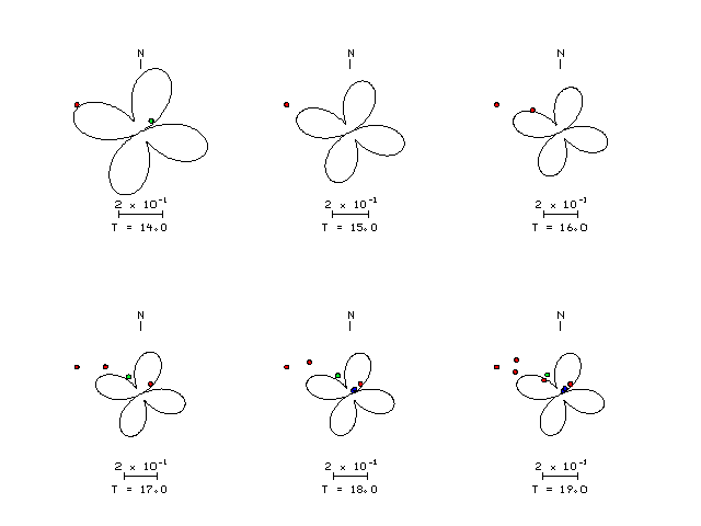
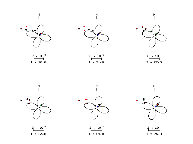
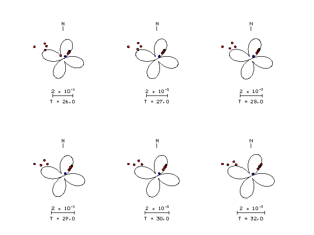
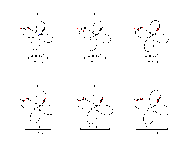
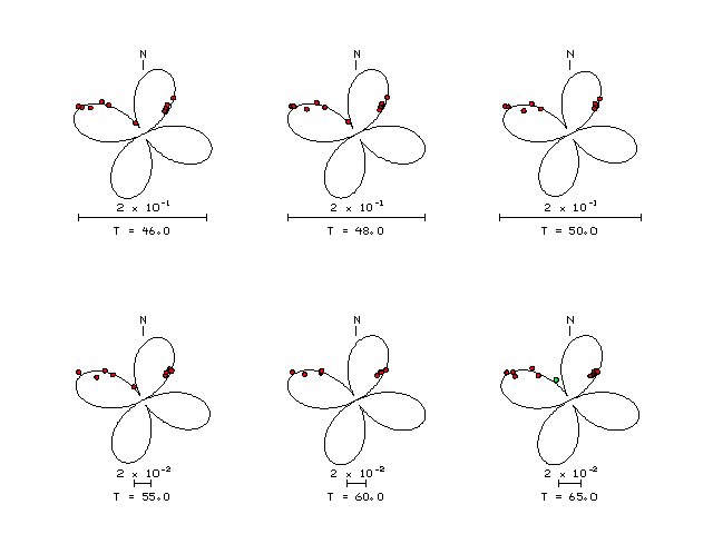
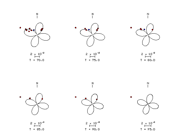
Focal mechanism sensitivity at the preferred depth. The red color indicates a very good fit to the Love and Rayleigh wave radiation patterns. Each solution is plotted as a vector at a given value of strike and dip with the angle of the vector representing the rake angle, measured, with respect to the upward vertical (N) in the figure. Because of the symmetry of the spectral amplitude rediation patterns, only strikes from 0-180 degrees are sampled.

Love-wave radiation patterns

Rayleigh-wave radiation patterns

Broadband station distributiuon

Sta Az(deg)    Dist(km)   
GNI	  328	 1785
MALT	  312	 2056
KSDI	  294	 2059
CSS	  298	 2318
AML	   40	 2338
EKS2	   38	 2382
UCH	   40	 2397
KZA	   42	 2435
KBK	   40	 2455
USP	   38	 2471
ULHL	   42	 2512
TKM2	   40	 2515
ANTO	  310	 2564
LAST	  295	 3022
IDI	  295	 3077
VOS	   20	 3125
BRVK	   19	 3135
GVD	  294	 3143
KURK	   30	 3268
ARU	    3	 3281
VTS	  309	 3421
LSA	   77	 3461
KIEV	  327	 3468
OBN	  339	 3495
KMBO	  216	 3690
DIVS	  310	 3723
TIP	  301	 3857
PSZ	  316	 3884
MBAR	  225	 4063

Waveform comparison for this mechanism

Since the analysis of the surface-wave radiation patterns uses only spectral amplitudes and because the surfave-wave radiation patterns have a 180 degree symmetry, each surface-wave solution consists of four possible focal mechanisms corresponding to the interchange of the P- and T-axes and a roation of the mechanism by 180 degrees. To select one mechanism, P-wave first motion can be used. This was not possible in this case because all the P-wave first motions were emergent ( a feature of the P-wave wave takeoff angle, the station location and the mechanism). The other way to select among the mechanisms is to compute forward synthetics and compare the observed and predicted waveforms.

The velocity model used for the waveform fit is a modified Utah model .

The fits to the waveforms with the given mechanism are show below:

This figure shows the fit to the three components of motion (Z - vertical, R-radial and T - transverse). For each station and component, the observed traces is shown in red and the model predicted trace in blue. The traces represent filtered ground velocity in units of meters/sec (the peak value is printed adjacent to each trace; each pair of traces to plotted to the same scale to emphasize the difference in levels). Both synthetic and observed traces have been filtered using the SAC commands:

hp c 0.01 3
lp c 0.05 3

Discussion

Appendix A

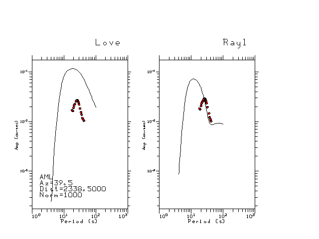
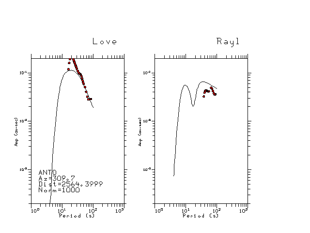
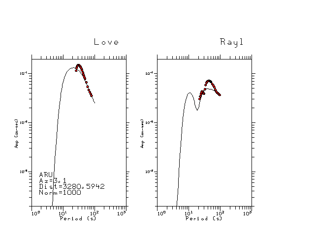
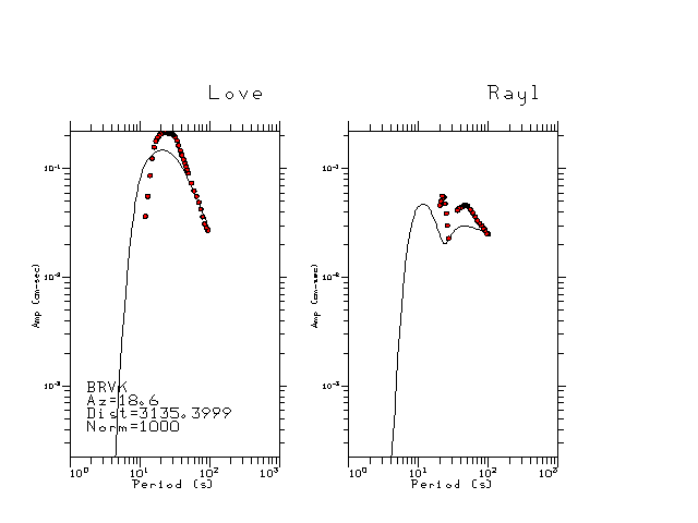
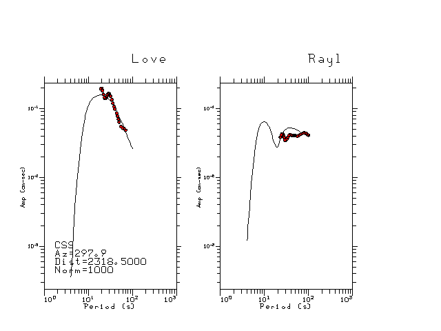
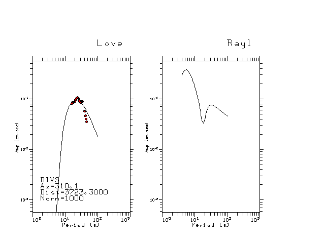
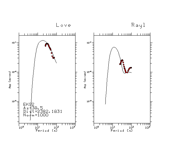
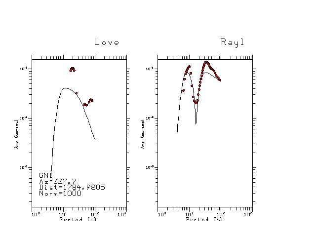
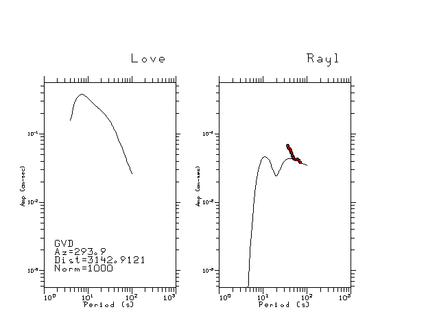
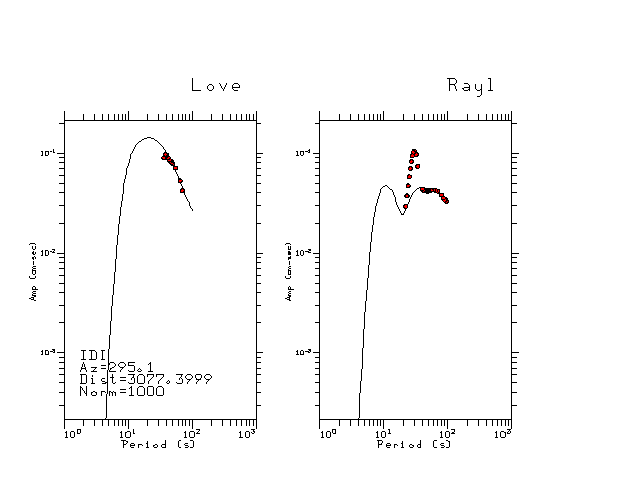
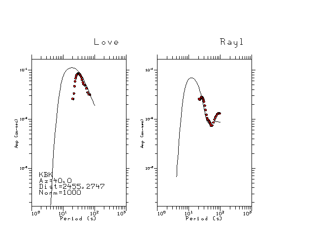
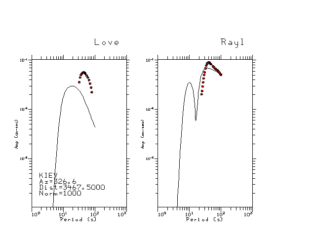
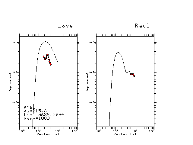
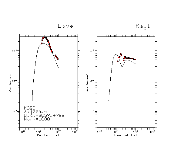
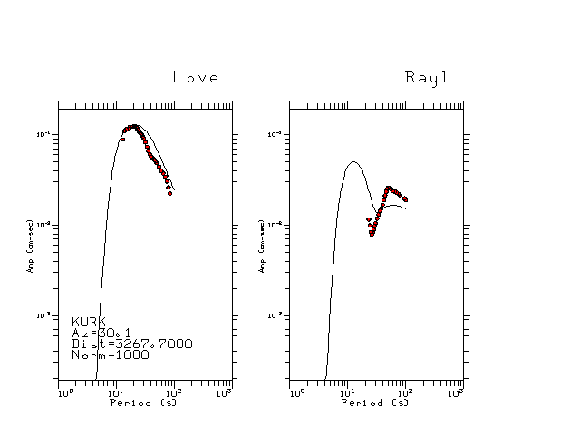
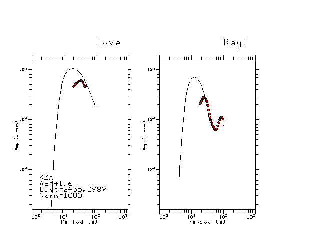
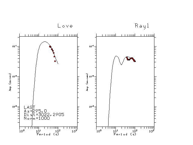
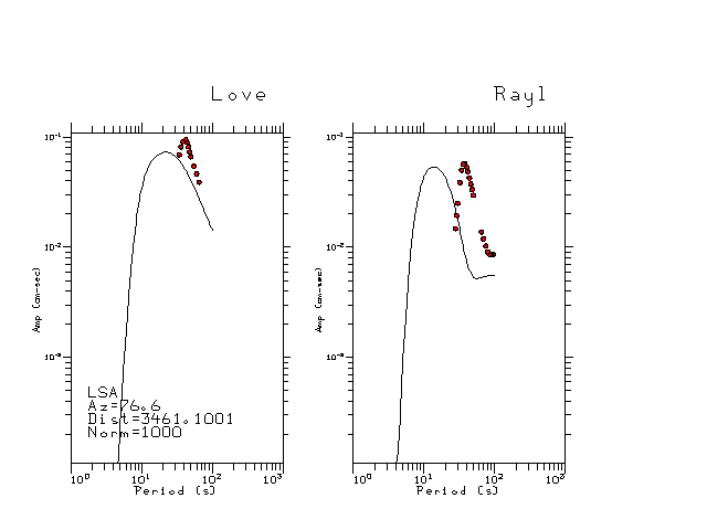
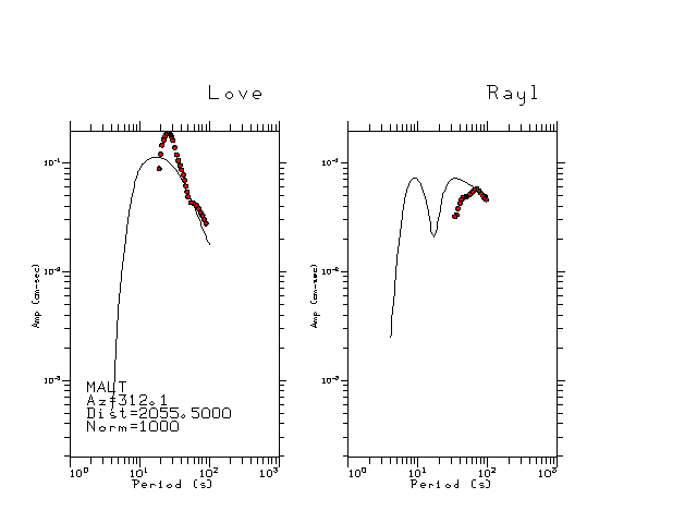
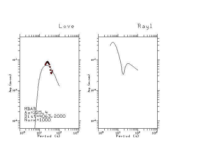
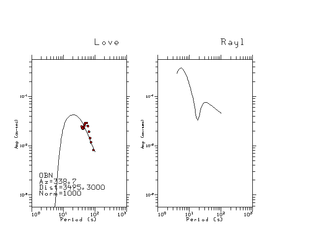
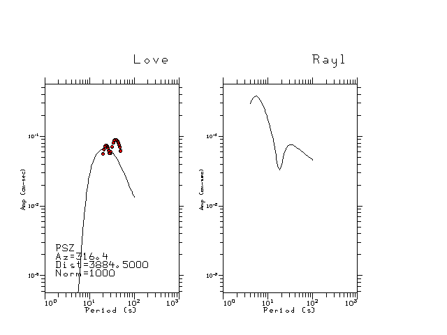
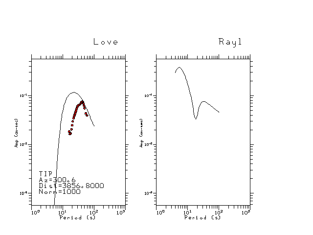
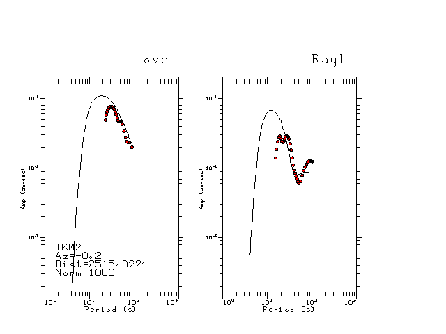
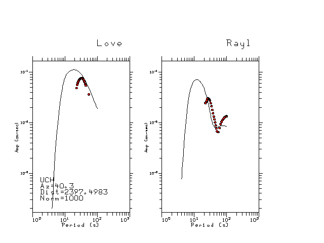
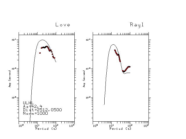
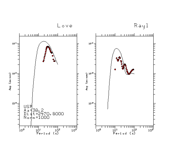
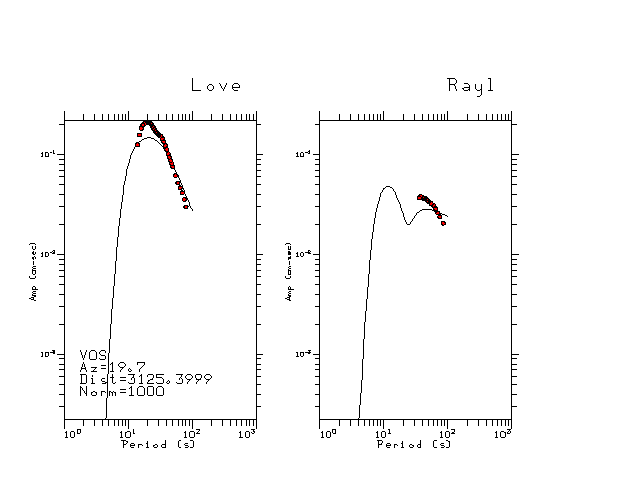
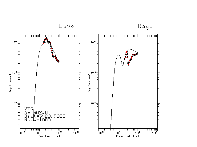
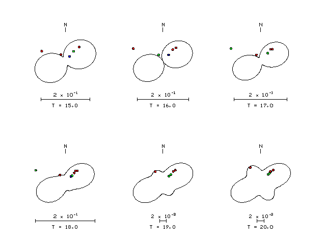
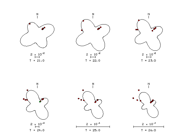
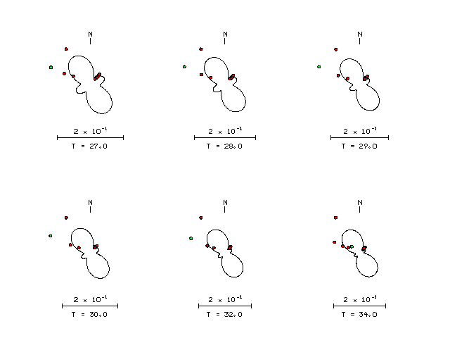
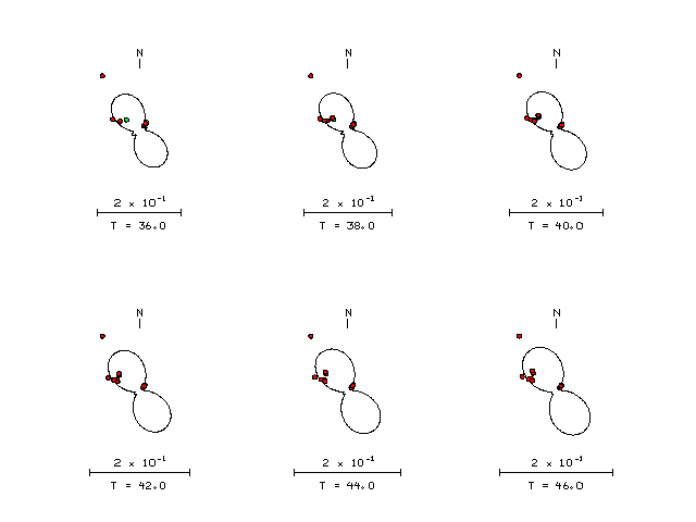
The figures below show the observed spectral amplitudes (units of cm-sec) at each station and the theoretical predictions as a function of period for the mechanism given above. The modified Utah model earth model was used to define the Green's functions. For each station, the Love and Rayleigh wave spectrail amplitudes are plotted with the same scaling so that one can get a sense fo the effects of the effects of the focal mechanism and depth on the excitation of each.

Last Changed 2006/06/29