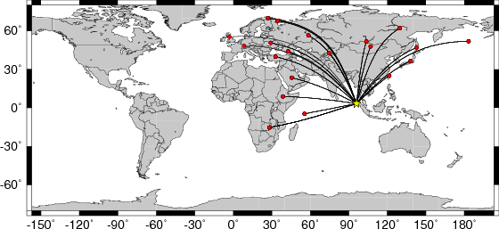
Location of the earthquake (yellow star) and great circle path from the epicenter to each station (red) [created using GMT (Wessel, P., and W. H. F. Smith, New version of Generic Mapping Tools released, EOS Trans. AGU, 76 329, 1995.)]
Thus solution is base on using a 200 second time window for this earthquake. A very long period filter was used - effoectively 200 to 250 seconds because of the filtering and the deconvolution. This inversion used the entire trace from P -30 to P + 2000 seconds. There is no attempt to model P, SH and SV phases, but rather the entire trace.
This example is also meant to test the ability of the Green's functions for a large earthquake.
2004/12/26 00:58:53 3.30 95.98 30
The following compares this source inversion to the USGS Rapid Moment Tensor Solution and to the Harvard CMT solutions, if they are available.
 SLU Moment Tensor Solution
 2004/12/26 00:58:53

 Best Fitting Double Couple
    Mo = 5.19e+28 dyne-cm
    Mw = 8.41
    Z  = 40 km
     Plane   Strike  Dip  Rake
      NP1      150    50    90
      NP2      330    40    90
 Principal Axes:
   Axis    Value   Plunge  Azimuth
     T   5.19e+28     85      60
     N   0.00e+00     -0     150
     P  -5.19e+28      5     240


 Moment Tensor: (dyne-cm)
    Component  Value
       Mxx    -1.28e+28
       Mxy    -2.21e+28
       Mxz     4.50e+27
       Myy    -3.83e+28
       Myz     7.80e+27
       Mzz     5.11e+28


                     --------------
                 #######---------------
              ---############-------------
             ---################-----------
           -----##################-----------
          -----#####################----------
         ------######################----------
        --------#######################---------
        --------########################--------
       ---------############   #########---------
       ----------########### T ##########--------
       ----------###########   ###########-------
       -----------########################-------
        -----------#######################------
        ------------######################------
            ----------####################-----
          P -----------###################----
            -------------################----
             --------------##############--
              ----------------##########--
                 ------------------####
                     --------------


 Harvard Convention
 Moment Tensor:
      R          T          F
  5.11e+28   4.50e+27  -7.80e+27
  4.50e+27  -1.28e+28   2.21e+28
 -7.80e+27   2.21e+28  -3.83e+28
|
04/12/26 00:58:50.76
 OFF W COAST OF NORTHERN SUMATRA
 Epicenter:   3.298   95.778
 MW 8.2

 USGS MOMENT TENSOR SOLUTION
 Depth   7         No. of sta: 31
 Moment Tensor;   Scale 10**21 Nm
   Mrr= 0.91       Mtt=-0.89
   Mff=-0.02       Mrt= 1.78
   Mrf=-1.55       Mtf= 0.47
  Principal axes:
   T  Val=  2.53  Plg=55  Azm= 50
   N        0.09       8      308
   P       -2.61      34      213

 Best Double Couple:Mo=2.6*10**21
  NP1:Strike=274 Dip=13 Slip=  55
  NP2:       130     79        98

               -------
          -----------------
        ---##############----
      --####################---
    ##-########################--
   #----########################--
   -------############   ########-
  ---------########### T #########-
  -----------#########   ##########
  -------------####################
  ---------------##################
  ------------------###############
   -------------------############
   --------   -----------#########
    ------- P --------------#####
      -----   -----------------
        ---------------------
          -----------------
               -------
|
ecember 26, 2004, OFF W COAST OF NORTHERN SUMATRA, MW=9.0

Meredith Nettles
Goran Ekstrom

CENTROID, MOMENT TENSOR SOLUTION
HARVARD EVENT-FILE NAME M122604A
DATA USED: GSN
MANTLE WAVES:    73S,202C, T=300
CENTROID LOCATION:
ORIGIN TIME       01:01: 9.0 0.3
LAT  3.09N 0.04;LON  94.26E 0.03
DEP  28.6 1.3;HALF-DURATION 95.0
MOMENT TENSOR; SCALE 10**29 D-CM
  MRR= 1.04 0.01; MTT=-0.43 0.01
  MPP=-0.61 0.01; MRT= 2.98 0.16
  MRP=-2.40 0.16; MTP= 0.43 0.00
 PRINCIPAL AXES:
 1.(T) VAL=  4.01;PLG=52;AZM= 36
 2.(N)      -0.12;     3;    130
 3.(P)      -3.89;    38;    222
BEST DOUBLE COUPLE:M0=4.0*10**29
 NP1:STRIKE=329;DIP= 8;SLIP= 110
 NP2:STRIKE=129;DIP=83;SLIP=  87

            -#######---
        #################--
      #####################--
    -########################--
   ----#############   #######--
  ------############ T ########--
  --------##########   #########-
 -----------#####################-
 -------------###################-
 ---------------#################-
 ------------------##############-
  -------------------############
  -------   ------------########-
   ------ P --------------#####-
    -----   -------------------
      -----------------------
        -------------------
            -----------
|
The following broadband stations passed the QC and were used for the source inversion. AAK ADK ANTO ARU BFO ESK FURI KEV KIEV KIV LSZ LVZ MAJO MSEY RAYN TATO TLY ULN YAK YSS
All observed and Greens function waveforms are corrected to instrument response to ground velocity in meters/sec for the passband of 0.004 - 5 Hz. The traces were then lowpass filtered at 0.25 Hz and interpolated to a sample rate of 1 second.
For the grid search, the observed traces and Green's functions are read in an cut using the following commands
Phase    Gsac Command              Comment
 P    cut A -30 A       CUTH = 95+0.3*DEPTH
SH    cut T1 -60 T1     CUTH = 95+0.6*DEPTH
SV    cut T0 -60 T0     CUTH = 95+0.6*DEPTH

where the 95 is a maximum filter duration, DEPTH is in km, and the CUTH in sec
The cut windows attempt to include the P, pP, sP, pS, S and sS arrivals. However, oen must be very careful about the fact that PP may be included in some distance ranges.
The waveforms are then bandpass filtered by the application of the following high- and low-pass stages (an optional microseism filter):
hp c 0.0020 2
lp c 0.0050 2
int
The traces were next integrated to ground displacment in meters. Finally the observed data are interpolated to ahve the same sampling at the Green's functions.
The source inversion is a multipass operation since a lower frequency filter band is used for larger earthquakes and since a search is made over depth. Up to three passed of the outer loop are made, after which the moment magnitude is determined and filter settings readjusted. The inner loop over depth samples all depths from 0 to 800 km with 5 km increments in depth to 50 km, followed by 10 km depth sampling for the remaining range.
The following filter ranges are used according to the moment magnitude Mw:
   FILTER_BAND   FH(s)  FL(s)
       1           60     12      Mw < 6.4
       2          100     20      6.4 < Mw <= 6.9
       3          120     40      Mw > 6.9
The map displays the distribution of stations used for this source inversion.
|
Location of the earthquake (yellow star) and great circle path from the epicenter to each station (red) [created using GMT (Wessel, P., and W. H. F. Smith, New version of Generic Mapping Tools released, EOS Trans. AGU, 76 329, 1995.)] |
For this data set the favored solution is
WVFGRD96 40.0 150 50 90 8.41 0.5369
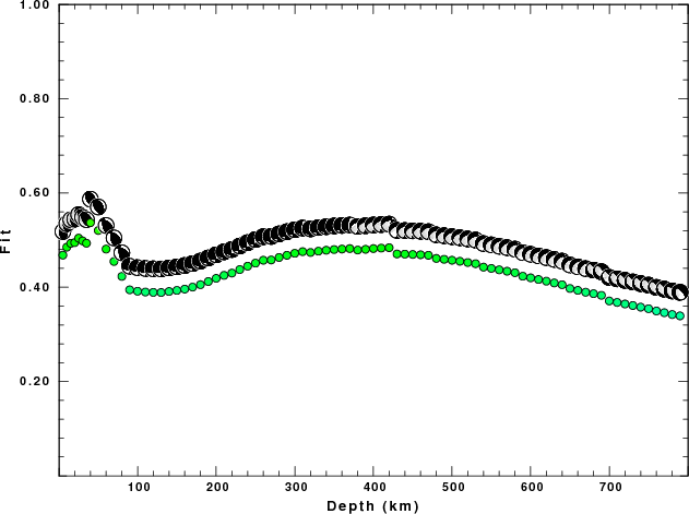
The following figures show the sensitivity of the goodness of fit parameter so source depth, the waveform comparison as a function of epicentral distance in degrees and the source to station azimuth
|
| Goodness of fit as a function of source depth. The measure is 1 - SUM (o -p)2 / SUM o2. A value of 1.0 is the best fit. The best double couple mechanism for the solution depth is plotted above goodness of fit value to indicate how the mefhanism may change with depth. |
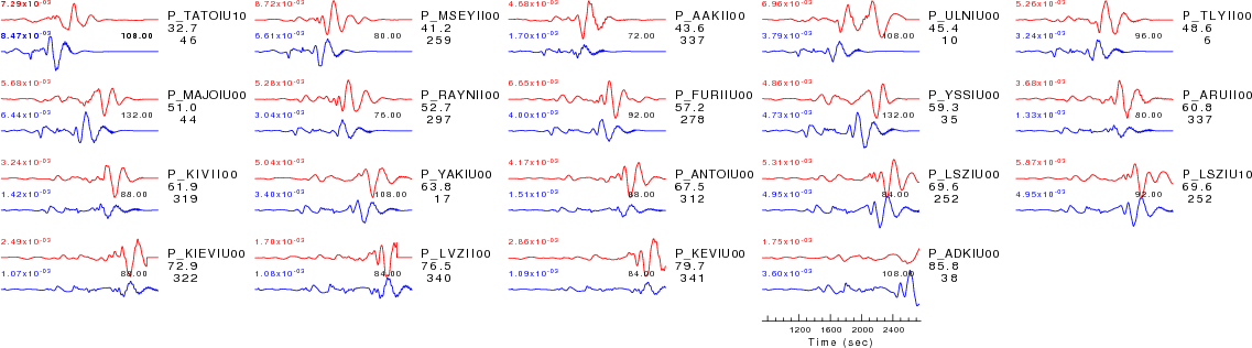
| P-wave Z component |
|
| Comparison of the observed traces (red) and solution predicted traces (blue) ordered in terms of increasing epicentral distance. Each pair of traces is annotated with the station name, epicentral distance in degrees, source to station azimuth in degrees. Each pair of traces is plotted with the same scale and the peak amplitudes are indicated at the lect of each trace. Finally the time shift between the P-wave first arrival picked and the the theoretical P-wave first arrival in the predicted trace is indicated, with a positive sign indicating that the predicted trace has been shifted to the right by the given number of seconds. as a function of source to station azimuth in degrees (D). The purpose of this display is to highlight the azimuthal dependence on the first motion. The traces are annotated with the station name at the top. |
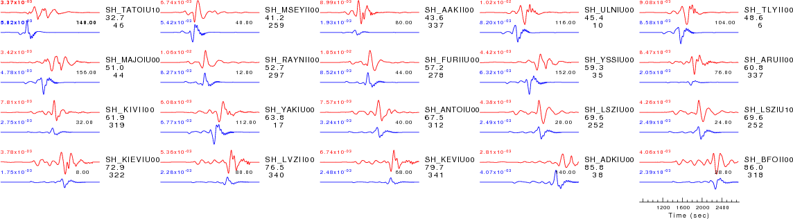
| SH-wave T component |
|
| Comparison of the observed traces (red) and solution predicted traces (blue) ordered in terms of increasing epicentral distance. Each pair of traces is annotated with the station name, epicentral distance in degrees, source to station azimuth in degrees. Each pair of traces is plotted with the same scale and the peak amplitudes are indicated at the lect of each trace. Finally the time shift between the P-wave first arrival picked and the the theoretical P-wave first arrival in the predicted trace is indicated, with a positive sign indicating that the predicted trace has been shifted to the right by the given number of seconds. as a function of source to station azimuth in degrees (D). The purpose of this display is to highlight the azimuthal dependence on the first motion. The traces are annotated with the station name at the top. |
| SV-wave R component |
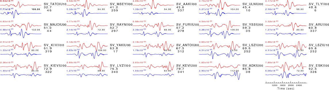
|
| Comparison of the observed traces (red) and solution predicted traces (blue) ordered in terms of increasing epicentral distance. Each pair of traces is annotated with the station name, epicentral distance in degrees, source to station azimuth in degrees. Each pair of traces is plotted with the same scale and the peak amplitudes are indicated at the lect of each trace. Finally the time shift between the P-wave first arrival picked and the the theoretical P-wave first arrival in the predicted trace is indicated, with a positive sign indicating that the predicted trace has been shifted to the right by the given number of seconds. as a function of source to station azimuth in degrees (D). The purpose of this display is to highlight the azimuthal dependence on the first motion. The traces are annotated with the station name at the top. |