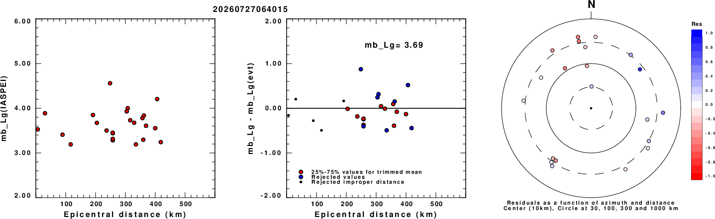
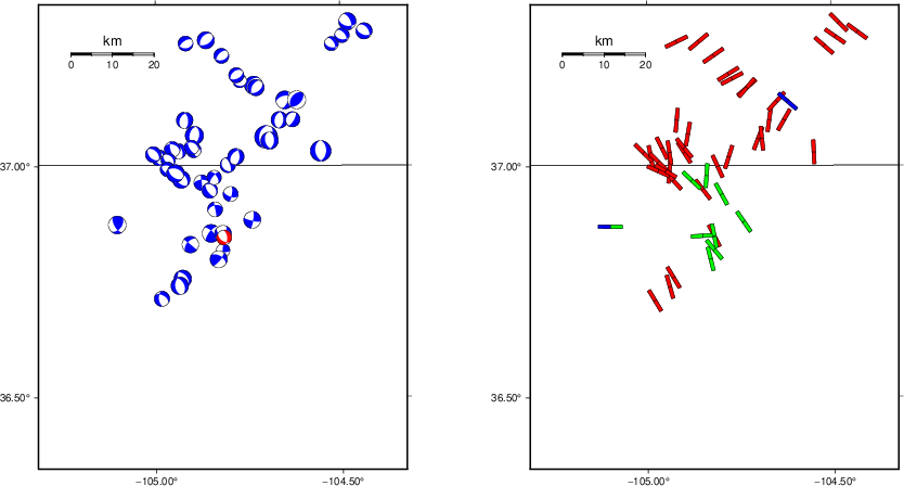
Left: mb_Lg computed using the IASPEI formula. Center: mb_Lg residuals versus epicentral distance ; the values used for the trimmed mean magnitude estimate are indicated. Right: residuals as a function of distance and azimuth.
The ANSS event ID is us7000t3lr and the event page is at https://earthquake.usgs.gov/earthquakes/eventpage/us7000t3lr/executive.
2026/07/27 06:40:15 36.846 -104.816 5.0 3.8 New Mexico
 USGS/SLU Moment Tensor Solution
 ENS  2026/07/27 06:40:15.0  36.85 -104.82   5.0 3.8 New Mexico

 Stations used:
   C0.LAMA C0.Q24A C0.S22A C0.YECK IU.ANMO N4.KSCO TX.RTBA
   US.SDCO YX.UNM5

 Filtering commands used:
   cut o DIST/3.3 -40 o DIST/3.3 +50
   rtr
   taper w 0.1
   hp c 0.03 n 3
   lp c 0.10 n 3

 Best Fitting Double Couple
  Mo = 1.76e+21 dyne-cm
  Mw = 3.43
  Z  = 6 km
  Plane   Strike  Dip  Rake
   NP1      355    55   -55
   NP2      124    48   -129
  Principal Axes:
   Axis    Value   Plunge  Azimuth
    T   1.76e+21      4      61
    N   0.00e+00     28     153
    P  -1.76e+21     62     324

 Moment Tensor: (dyne-cm)
    Component   Value
       Mxx     1.54e+20
       Mxy     9.31e+20
       Mxz    -5.33e+20
       Myy     1.20e+21
       Myz     5.41e+20
       Mzz    -1.35e+21


                     -------#######
                 -------------#########
              ------------------##########
             --------------------##########
           -----------------------##########
          #------------------------######### T
         ##-----------   ----------#########
        ###----------- P -----------############
        ####----------   -----------############
       #####-------------------------############
       ######------------------------############
       #######-----------------------############
       #########---------------------############
        #########--------------------###########
        ###########------------------###########
         ############---------------###########
          ##############------------##########
           #################-------#########-
             ######################--------
              ####################--------
                 ################------
                     ##########----


 Global CMT Convention Moment Tensor:
      R          T          P
 -1.35e+21  -5.33e+20  -5.41e+20
 -5.33e+20   1.54e+20  -9.31e+20
 -5.41e+20  -9.31e+20   1.20e+21


Details of the solution is found at

http://www.eas.slu.edu/eqc/eqc_mt/MECH.NA/20260727064015/index.html
|
      STK = 355
      DIP = 55
     RAKE = -55
       MW = 3.43
       HS = 6.0
The NDK file is 20260727064015.ndk The waveform inversion is preferred.
Given the availability of digital waveforms for determination of the moment tensor, this section documents the added processing leading to mLg, if appropriate to the region, and ML by application of the respective IASPEI formulae. As a research study, the linear distance term of the IASPEI formula for ML is adjusted to remove a linear distance trend in residuals to give a regionally defined ML. The defined ML uses horizontal component recordings, but the same procedure is applied to the vertical components since there may be some interest in vertical component ground motions. Residual plots versus distance may indicate interesting features of ground motion scaling in some distance ranges. A residual plot of the regionalized magnitude is given as a function of distance and azimuth, since data sets may transcend different wave propagation provinces.
Left: mb_Lg computed using the IASPEI formula. Center: mb_Lg residuals versus epicentral distance ; the values used for the trimmed mean magnitude estimate are indicated.
Right: residuals as a function of distance and azimuth.
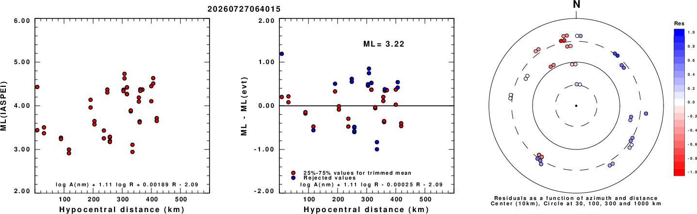
Left: ML computed using the IASPEI formula for Horizontal components. Center: ML residuals computed using a modified IASPEI formula that accounts for path specific attenuation; the values used for the trimmed mean are indicated. The ML relation used for each figure is given at the bottom of each plot.
Right: Residuals from new relation as a function of distance and azimuth.
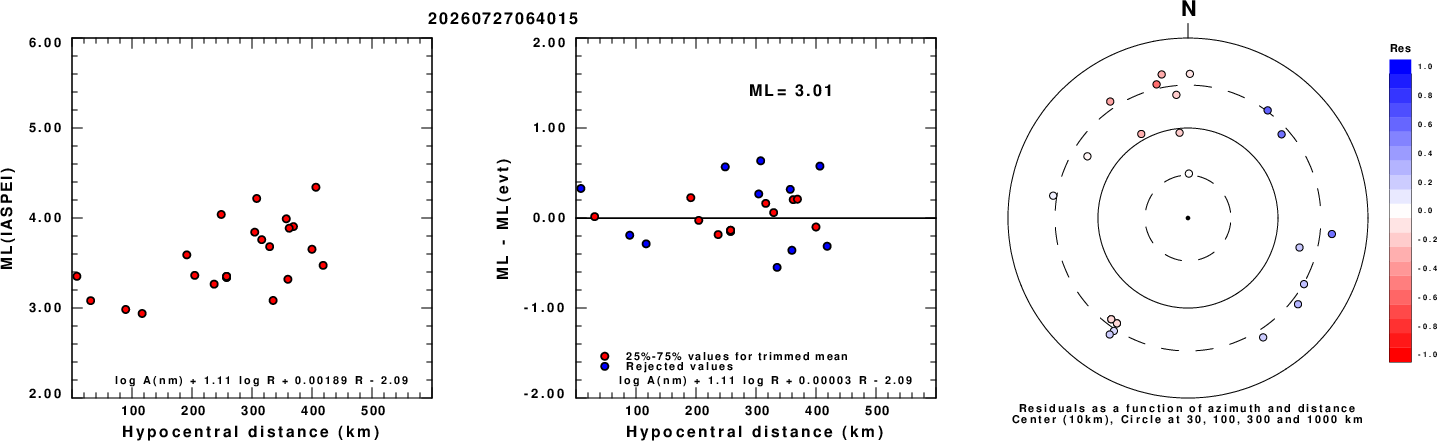
Left: ML computed using the IASPEI formula for Vertical components (research). Center: ML residuals computed using a modified IASPEI formula that accounts for path specific attenuation; the values used for the trimmed mean are indicated. The ML relation used for each figure is given at the bottom of each plot.
Right: Residuals from new relation as a function of distance and azimuth.
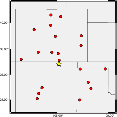
Map showing station locations used for computing the ML's. No distinction is made whether the vertical (Z) or horizontal (H) components were used.
 |
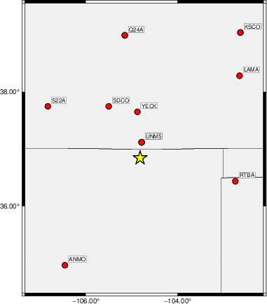
The focal mechanism was determined using broadband seismic waveforms. The location of the event (star) and the stations used for (red) the waveform inversion are shown in the next figure.
|
|
|
The program wvfgrd96 was used with good traces observed at short distance to determine the focal mechanism, depth and seismic moment. This technique requires a high quality signal and well determined velocity model for the Green's functions. To the extent that these are the quality data, this type of mechanism should be preferred over the radiation pattern technique which requires the separate step of defining the pressure and tension quadrants and the correct strike.
The observed and predicted traces are filtered using the following gsac commands:
cut o DIST/3.3 -40 o DIST/3.3 +50
rtr
taper w 0.1
hp c 0.03 n 3
lp c 0.10 n 3
The results of this grid search are as follow:
           DEPTH  STK   DIP  RAKE   MW    FIT
WVFGRD96    1.0   155    80    15   3.17 0.3241
WVFGRD96    2.0   160    70    25   3.33 0.3789
WVFGRD96    3.0    10    45   -25   3.32 0.4177
WVFGRD96    4.0   355    55   -60   3.41 0.4789
WVFGRD96    5.0   350    50   -60   3.42 0.5174
WVFGRD96    6.0   355    55   -55   3.43 0.5284
WVFGRD96    7.0   355    60   -55   3.45 0.5203
WVFGRD96    8.0   355    55   -60   3.53 0.5188
WVFGRD96    9.0    -5    60   -60   3.54 0.4991
WVFGRD96   10.0    -5    65   -55   3.55 0.4771
WVFGRD96   11.0     0    65   -50   3.55 0.4532
WVFGRD96   12.0     0    70   -45   3.55 0.4329
WVFGRD96   13.0   200    75    45   3.56 0.4206
WVFGRD96   14.0   200    75    40   3.56 0.4055
WVFGRD96   15.0   195    80    35   3.58 0.3903
WVFGRD96   16.0   195    80    35   3.59 0.3808
WVFGRD96   17.0   195    80    35   3.60 0.3722
WVFGRD96   18.0   185    75    30   3.62 0.3638
WVFGRD96   19.0    15    85   -30   3.63 0.3569
WVFGRD96   20.0    15    85   -30   3.64 0.3523
WVFGRD96   21.0    15    70   -15   3.61 0.3494
WVFGRD96   22.0    15    70   -10   3.61 0.3467
WVFGRD96   23.0    15    70   -10   3.61 0.3440
WVFGRD96   24.0    20    65    -5   3.62 0.3423
WVFGRD96   25.0    20    65    -5   3.62 0.3412
WVFGRD96   26.0    20    65    -5   3.63 0.3413
WVFGRD96   27.0    20    70   -10   3.66 0.3423
WVFGRD96   28.0    20    70   -10   3.67 0.3419
WVFGRD96   29.0    20    70   -10   3.68 0.3434
The best solution is
WVFGRD96 6.0 355 55 -55 3.43 0.5284
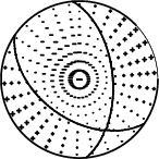
The mechanism corresponding to the best fit is
|
|
|
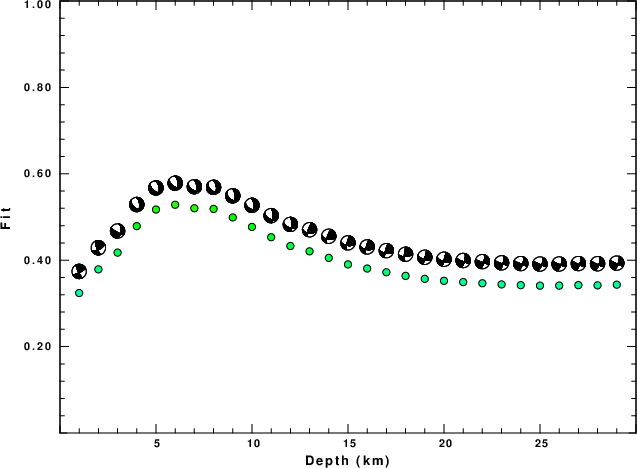
The best fit as a function of depth is given in the following figure:
|
|
|
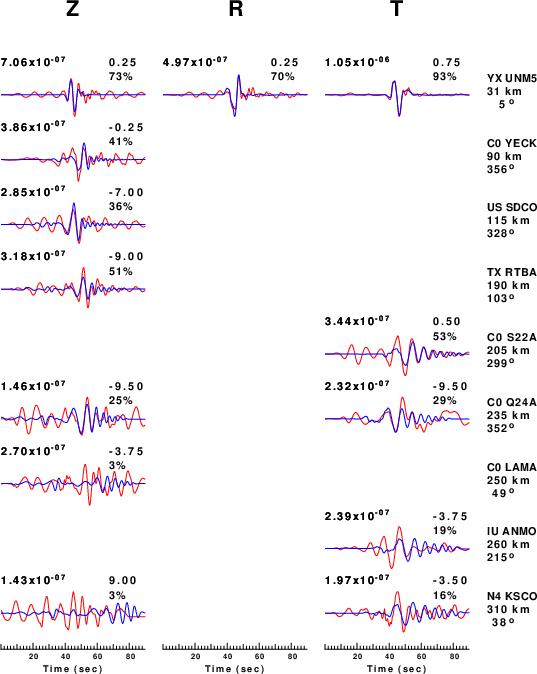
The comparison of the observed and predicted waveforms is given in the next figure. The red traces are the observed and the blue are the predicted. Each observed-predicted component is plotted to the same scale and peak amplitudes are indicated by the numbers to the left of each trace. A pair of numbers is given in black at the right of each predicted traces. The upper number it the time shift required for maximum correlation between the observed and predicted traces. This time shift is required because the synthetics are not computed at exactly the same distance as the observed, the velocity model used in the predictions may not be perfect and the epicentral parameters may be be off. A positive time shift indicates that the prediction is too fast and should be delayed to match the observed trace (shift to the right in this figure). A negative value indicates that the prediction is too slow. The lower number gives the percentage of variance reduction to characterize the individual goodness of fit (100% indicates a perfect fit).
The bandpass filter used in the processing and for the display was
cut o DIST/3.3 -40 o DIST/3.3 +50
rtr
taper w 0.1
hp c 0.03 n 3
lp c 0.10 n 3
|
| Figure 3. Waveform comparison for selected depth. Red: observed; Blue - predicted. The time shift with respect to the model prediction is indicated. The percent of fit is also indicated. The time scale is relative to the first trace sample. |
|
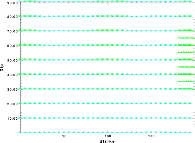
| Focal mechanism sensitivity at the preferred depth. The red color indicates a very good fit to the waveforms. Each solution is plotted as a vector at a given value of strike and dip with the angle of the vector representing the rake angle, measured, with respect to the upward vertical (N) in the figure. |
A check on the assumed source location is possible by looking at the time shifts between the observed and predicted traces. The time shifts for waveform matching arise for several reasons:
Time_shift = A + B cos Azimuth + C Sin Azimuth
The time shifts for this inversion lead to the next figure:
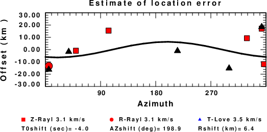
The derived shift in origin time and epicentral coordinates are given at the bottom of the figure.
The WUS.model used for the waveform synthetic seismograms and for the surface wave eigenfunctions and dispersion is as follows (The format is in the model96 format of Computer Programs in Seismology).
MODEL.01
Model after     8 iterations
ISOTROPIC
KGS
FLAT EARTH
1-D
CONSTANT VELOCITY
LINE08
LINE09
LINE10
LINE11
      H(KM)   VP(KM/S)   VS(KM/S) RHO(GM/CC)         QP         QS       ETAP       ETAS      FREFP      FREFS
     1.9000     3.4065     2.0089     2.2150  0.302E-02  0.679E-02   0.00       0.00       1.00       1.00
     6.1000     5.5445     3.2953     2.6089  0.349E-02  0.784E-02   0.00       0.00       1.00       1.00
    13.0000     6.2708     3.7396     2.7812  0.212E-02  0.476E-02   0.00       0.00       1.00       1.00
    19.0000     6.4075     3.7680     2.8223  0.111E-02  0.249E-02   0.00       0.00       1.00       1.00
     0.0000     7.9000     4.6200     3.2760  0.164E-10  0.370E-10   0.00       0.00       1.00       1.00