Location
Location ANSS
The ANSS event ID is us6000sq0v and the event page is at
https://earthquake.usgs.gov/earthquakes/eventpage/us6000sq0v/executive.
2026/04/14 16:36:42 45.768 -76.397 10.0 4.0 Ontario, Canada
Focal Mechanism
 USGS/SLU Moment Tensor Solution
 ENS  2026/04/14 16:36:42.0  45.77  -76.40  10.0 4.0 Ontario, Canada

 Stations used:
   CN.A16 CN.A54 CN.DPQ CN.KGNO CN.LDAQ CN.LMQ CN.MNTQ CN.SADO
   CN.TRQ CN.VLDQ CN.WBO IU.HRV LD.BRNY LD.CCNY LD.FLET
   LD.KSPA LD.ODNJ LD.PRNY LD.UNH N4.G62A N4.H62A N4.I62A
   N4.I63A N4.J55A N4.J57A N4.J59A N4.J61A N4.K57A N4.K62A
   N4.L56A N4.L59A N4.L61B N4.M57A NE.HNH NE.TRY NE.VT1
   PE.PABE PE.PALR PE.PAMP PE.PAOC PE.PSWB US.BINY US.LBNH
   US.LONY WU.ACTO WU.BMRO WU.BUKO WU.CLWO WU.DELO WU.ELFO
   WU.KLBO WU.PECO WU.PEMO WU.PKRO2 WU.PLVO WU.TOBO WU.TYNO
   WU.WLVO

 Filtering commands used:
   cut o DIST/3.3 -30 o DIST/3.3 +40
   rtr
   taper w 0.1
   hp c 0.03 n 3
   lp c 0.10 n 3

 Best Fitting Double Couple
  Mo = 1.14e+22 dyne-cm
  Mw = 3.97
  Z  = 12 km
  Plane   Strike  Dip  Rake
   NP1      355    55   120
   NP2      130    45    55
  Principal Axes:
   Axis    Value   Plunge  Azimuth
    T   1.14e+22     65     323
    N   0.00e+00     24     156
    P  -1.14e+22      5      64

 Moment Tensor: (dyne-cm)
    Component   Value
       Mxx    -9.23e+20
       Mxy    -5.38e+21
       Mxz     2.96e+21
       Myy    -8.37e+21
       Myz    -3.53e+21
       Mzz     9.30e+21


                     #######-------
                 #############---------
              ##################----------
             ####################----------
           -######################-----------
          --#######################---------
         ---#######################--------- P
        ----###########   ##########--------   -
        ----########### T ##########------------
       ------##########   ###########------------
       ------########################------------
       -------#######################------------
       ---------#####################------------
        ---------####################-----------
        -----------##################-----------
         -----------################-----------
          -------------#############----------
           ---------------##########---------
             -----------------#####--------
              --------------------########
                 ----------------######
                     ----------####


 Global CMT Convention Moment Tensor:
      R          T          P
  9.30e+21   2.96e+21   3.53e+21
  2.96e+21  -9.23e+20   5.38e+21
  3.53e+21   5.38e+21  -8.37e+21


Details of the solution is found at

http://www.eas.slu.edu/eqc/eqc_mt/MECH.NA/20260414163642/index.html
|
Preferred Solution
The preferred solution from an analysis of the surface-wave spectral amplitude radiation pattern, waveform inversion or first motion observations is
      STK = 130
      DIP = 45
     RAKE = 55
       MW = 3.97
       HS = 12.0
The NDK file is 20260414163642.ndk
The waveform inversion is preferred.
Moment Tensor Comparison
The following compares this source inversion to those provided by others. The purpose is to look for major differences and also to note slight differences that might be inherent to the processing procedure. For completeness the USGS/SLU solution is repeated from above.
| SLU |
USGSMWR |
 USGS/SLU Moment Tensor Solution
 ENS  2026/04/14 16:36:42.0  45.77  -76.40  10.0 4.0 Ontario, Canada

 Stations used:
   CN.A16 CN.A54 CN.DPQ CN.KGNO CN.LDAQ CN.LMQ CN.MNTQ CN.SADO
   CN.TRQ CN.VLDQ CN.WBO IU.HRV LD.BRNY LD.CCNY LD.FLET
   LD.KSPA LD.ODNJ LD.PRNY LD.UNH N4.G62A N4.H62A N4.I62A
   N4.I63A N4.J55A N4.J57A N4.J59A N4.J61A N4.K57A N4.K62A
   N4.L56A N4.L59A N4.L61B N4.M57A NE.HNH NE.TRY NE.VT1
   PE.PABE PE.PALR PE.PAMP PE.PAOC PE.PSWB US.BINY US.LBNH
   US.LONY WU.ACTO WU.BMRO WU.BUKO WU.CLWO WU.DELO WU.ELFO
   WU.KLBO WU.PECO WU.PEMO WU.PKRO2 WU.PLVO WU.TOBO WU.TYNO
   WU.WLVO

 Filtering commands used:
   cut o DIST/3.3 -30 o DIST/3.3 +40
   rtr
   taper w 0.1
   hp c 0.03 n 3
   lp c 0.10 n 3

 Best Fitting Double Couple
  Mo = 1.14e+22 dyne-cm
  Mw = 3.97
  Z  = 12 km
  Plane   Strike  Dip  Rake
   NP1      355    55   120
   NP2      130    45    55
  Principal Axes:
   Axis    Value   Plunge  Azimuth
    T   1.14e+22     65     323
    N   0.00e+00     24     156
    P  -1.14e+22      5      64

 Moment Tensor: (dyne-cm)
    Component   Value
       Mxx    -9.23e+20
       Mxy    -5.38e+21
       Mxz     2.96e+21
       Myy    -8.37e+21
       Myz    -3.53e+21
       Mzz     9.30e+21


                     #######-------
                 #############---------
              ##################----------
             ####################----------
           -######################-----------
          --#######################---------
         ---#######################--------- P
        ----###########   ##########--------   -
        ----########### T ##########------------
       ------##########   ###########------------
       ------########################------------
       -------#######################------------
       ---------#####################------------
        ---------####################-----------
        -----------##################-----------
         -----------################-----------
          -------------#############----------
           ---------------##########---------
             -----------------#####--------
              --------------------########
                 ----------------######
                     ----------####


 Global CMT Convention Moment Tensor:
      R          T          P
  9.30e+21   2.96e+21   3.53e+21
  2.96e+21  -9.23e+20   5.38e+21
  3.53e+21   5.38e+21  -8.37e+21


Details of the solution is found at

http://www.eas.slu.edu/eqc/eqc_mt/MECH.NA/20260414163642/index.html
|
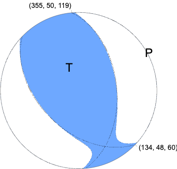
Regional Moment Tensor (Mwr)
Moment 1.242e+15 N-m
Magnitude 4.00 Mwr
Depth 13.0 km
Percent DC 90%
Half Duration -
Catalog US
Data Source US
Contributor US

Nodal Planes
Plane	Strike	Dip	Rake
NP1	355	50	119
NP2	134	48	60
Principal Axes
Axis	Value	Plunge	Azimuth
T	1.211e+15	68	333
N	0.061e+15	22	155
P	-1.271e+15	1	65
|
Magnitudes
Given the availability of digital waveforms for determination of the moment tensor, this section documents the added processing leading to mLg, if appropriate to the region, and ML by application of the respective IASPEI formulae. As a research study, the linear distance term of the IASPEI formula
for ML is adjusted to remove a linear distance trend in residuals to give a regionally defined ML. The defined ML uses horizontal component recordings, but the same procedure is applied to the vertical components since there may be some interest in vertical component ground motions. Residual plots versus distance may indicate interesting features of ground motion scaling in some distance ranges. A residual plot of the regionalized magnitude is given as a function of distance and azimuth, since data sets may transcend different wave propagation provinces.
mLg Magnitude
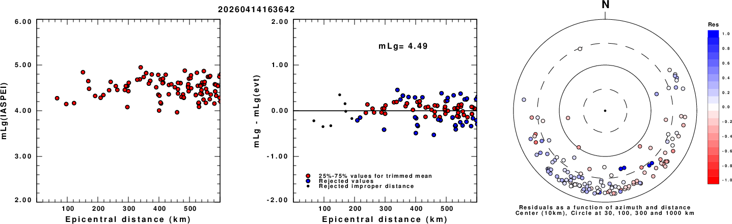
Left: mLg computed using the IASPEI formula. Center: mLg residuals versus epicentral distance ; the values used for the trimmed mean magnitude estimate are indicated.
Right: residuals as a function of distance and azimuth.
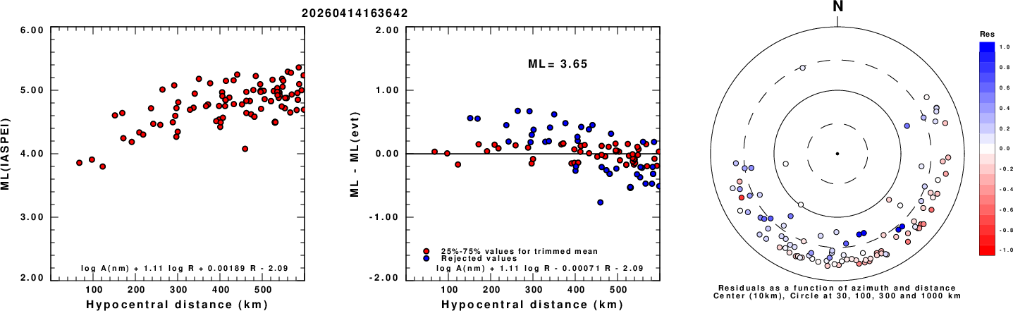
ML Magnitude
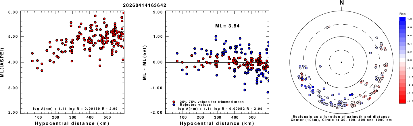
Left: ML computed using the IASPEI formula for Horizontal components. Center: ML residuals computed using a modified IASPEI formula that accounts for path specific attenuation; the values used for the trimmed mean are indicated. The ML relation used for each figure is given at the bottom of each plot.
Right: Residuals from new relation as a function of distance and azimuth.
Left: ML computed using the IASPEI formula for Vertical components (research). Center: ML residuals computed using a modified IASPEI formula that accounts for path specific attenuation; the values used for the trimmed mean are indicated. The ML relation used for each figure is given at the bottom of each plot.
Right: Residuals from new relation as a function of distance and azimuth.
Context
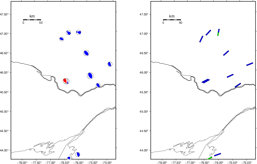
The left panel of the next figure presents the focal mechanism for this earthquake (red) in the context of other nearby events (blue) in the SLU Moment Tensor Catalog. The right panel shows the inferred direction of maximum compressive stress and the type of faulting (green is strike-slip, red is normal, blue is thrust; oblique is shown by a combination of colors). Thus context plot is useful for assessing the appropriateness of the moment tensor of this event.
Waveform Inversion using wvfgrd96
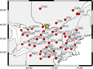
The focal mechanism was determined using broadband seismic waveforms. The location of the event (star) and the
stations used for (red) the waveform inversion are shown in the next figure.
|
|
Location of broadband stations used for waveform inversion
|
The program wvfgrd96 was used with good traces observed at short distance to determine the focal mechanism, depth and seismic moment. This technique requires a high quality signal and well determined velocity model for the Green's functions. To the extent that these are the quality data, this type of mechanism should be preferred over the radiation pattern technique which requires the separate step of defining the pressure and tension quadrants and the correct strike.
The observed and predicted traces are filtered using the following gsac commands:
cut o DIST/3.3 -30 o DIST/3.3 +40
rtr
taper w 0.1
hp c 0.03 n 3
lp c 0.10 n 3
The results of this grid search are as follow:
           DEPTH  STK   DIP  RAKE   MW    FIT
WVFGRD96    1.0    70    50   -90   3.84 0.4927
WVFGRD96    2.0   100    75   -60   3.92 0.5103
WVFGRD96    3.0   100    75   -55   3.89 0.5291
WVFGRD96    4.0   100    75   -55   3.88 0.5463
WVFGRD96    5.0   100    75   -55   3.88 0.5621
WVFGRD96    6.0   105    80   -50   3.87 0.5741
WVFGRD96    7.0   310    65    60   3.89 0.5931
WVFGRD96    8.0   315    60    65   3.90 0.6137
WVFGRD96    9.0   135    40    65   3.93 0.6296
WVFGRD96   10.0   130    45    60   3.96 0.6382
WVFGRD96   11.0   130    45    60   3.96 0.6464
WVFGRD96   12.0   130    45    55   3.97 0.6477
WVFGRD96   13.0   130    45    55   3.97 0.6445
WVFGRD96   14.0   120    50    45   3.98 0.6383
WVFGRD96   15.0   120    50    45   3.99 0.6298
WVFGRD96   16.0   120    50    45   3.99 0.6187
WVFGRD96   17.0   120    50    45   4.00 0.6054
WVFGRD96   18.0   120    50    45   4.01 0.5906
WVFGRD96   19.0   115    50    40   4.02 0.5747
WVFGRD96   20.0   120    45    45   4.04 0.5572
WVFGRD96   21.0   120    45    40   4.04 0.5416
WVFGRD96   22.0   120    45    40   4.05 0.5254
WVFGRD96   23.0   120    45    40   4.05 0.5080
WVFGRD96   24.0   120    40    40   4.06 0.4906
WVFGRD96   25.0   120    40    40   4.06 0.4735
WVFGRD96   26.0   120    40    35   4.07 0.4563
WVFGRD96   27.0   120    40    35   4.08 0.4405
WVFGRD96   28.0   120    40    35   4.08 0.4244
WVFGRD96   29.0   120    40    35   4.09 0.4080
The best solution is
WVFGRD96 12.0 130 45 55 3.97 0.6477
The mechanism corresponding to the best fit is
|
|
Figure 1. Waveform inversion focal mechanism
|
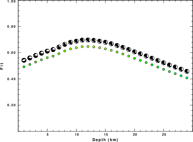
The best fit as a function of depth is given in the following figure:
|
|
Figure 2. Depth sensitivity for waveform mechanism
|
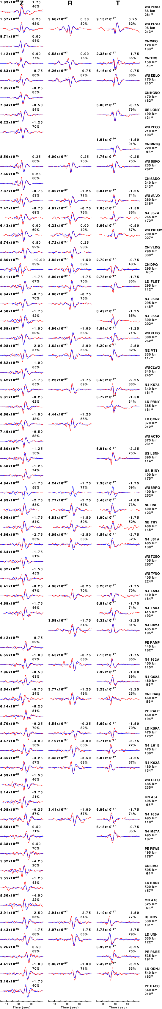
The comparison of the observed and predicted waveforms is given in the next figure. The red traces are the observed and the blue are the predicted.
Each observed-predicted component is plotted to the same scale and peak amplitudes are indicated by the numbers to the left of each trace. A pair of numbers is given in black at the right of each predicted traces. The upper number it the time shift required for maximum correlation between the observed and predicted traces. This time shift is required because the synthetics are not computed at exactly the same distance as the observed, the velocity model used in the predictions may not be perfect and the epicentral parameters may be be off.
A positive time shift indicates that the prediction is too fast and should be delayed to match the observed trace (shift to the right in this figure). A negative value indicates that the prediction is too slow. The lower number gives the percentage of variance reduction to characterize the individual goodness of fit (100% indicates a perfect fit).
The bandpass filter used in the processing and for the display was
cut o DIST/3.3 -30 o DIST/3.3 +40
rtr
taper w 0.1
hp c 0.03 n 3
lp c 0.10 n 3
|
|
Figure 3. Waveform comparison for selected depth. Red: observed; Blue - predicted. The time shift with respect to the model prediction is indicated. The percent of fit is also indicated. The time scale is relative to the first trace sample.
|
|
|
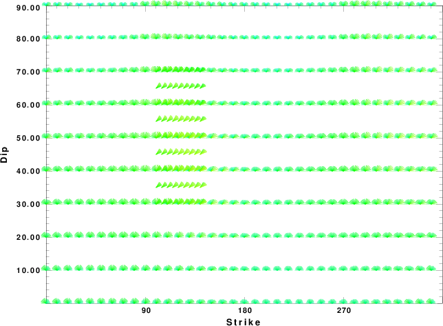
Focal mechanism sensitivity at the preferred depth. The red color indicates a very good fit to the waveforms.
Each solution is plotted as a vector at a given value of strike and dip with the angle of the vector representing the rake angle, measured, with respect to the upward vertical (N) in the figure.
|
A check on the assumed source location is possible by looking at the time shifts between the observed and predicted traces. The time shifts for waveform matching arise for several reasons:
- The origin time and epicentral distance are incorrect
- The velocity model used for the inversion is incorrect
- The velocity model used to define the P-arrival time is not the
same as the velocity model used for the waveform inversion
(assuming that the initial trace alignment is based on the
P arrival time)
Assuming only a mislocation, the time shifts are fit to a functional form:
Time_shift = A + B cos Azimuth + C Sin Azimuth
The time shifts for this inversion lead to the next figure:
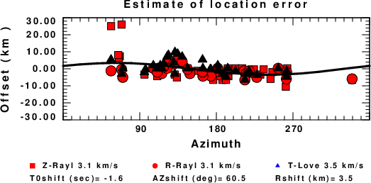
The derived shift in origin time and epicentral coordinates are given at the bottom of the figure.
Velocity Model
The CUS.model used for the waveform synthetic seismograms and for the surface wave eigenfunctions and dispersion is as follows
(The format is in the model96 format of Computer Programs in Seismology).
MODEL.01
CUS Model with Q from simple gamma values
ISOTROPIC
KGS
FLAT EARTH
1-D
CONSTANT VELOCITY
LINE08
LINE09
LINE10
LINE11
  H(KM) VP(KM/S) VS(KM/S) RHO(GM/CC)   QP   QS  ETAP  ETAS  FREFP  FREFS
  1.0000  5.0000  2.8900  2.5000 0.172E-02 0.387E-02 0.00  0.00  1.00  1.00
  9.0000  6.1000  3.5200  2.7300 0.160E-02 0.363E-02 0.00  0.00  1.00  1.00
 10.0000  6.4000  3.7000  2.8200 0.149E-02 0.336E-02 0.00  0.00  1.00  1.00
 20.0000  6.7000  3.8700  2.9020 0.000E-04 0.000E-04 0.00  0.00  1.00  1.00
  0.0000  8.1500  4.7000  3.3640 0.194E-02 0.431E-02 0.00  0.00  1.00  1.00
Last Changed Tue Apr 14 13:25:38 CDT 2026