Location
Location ANSS
The ANSS event ID is ak2026alfphj and the event page is at
https://earthquake.usgs.gov/earthquakes/eventpage/ak2026alfphj/executive.
2026/01/07 02:37:51 63.079 -150.989 127.0 4.5 Alaska
Focal Mechanism
 USGS/SLU Moment Tensor Solution
 ENS  2026/01/07 02:37:51.0  63.08 -150.99 127.0 4.5 Alaska

 Stations used:
   AK.BPAW AK.CAST AK.CCB AK.CUT AK.DHY AK.FIRE AK.GCSA AK.GHO
   AK.GLI AK.H24K AK.HDA AK.I23K AK.J19K AK.J20K AK.J25K
   AK.KNK AK.L19K AK.L22K AK.MCK AK.NEA2 AK.PAX AK.POKR
   AK.RC01 AK.SAW AK.SCM AK.SKN AK.WRH AT.PMR AV.STLK IM.IL31
   IU.COLA

 Filtering commands used:
   cut o DIST/3.5 -40 o DIST/3.5 +50
   rtr
   taper w 0.1
   hp c 0.03 n 3
   lp c 0.08 n 3

 Best Fitting Double Couple
  Mo = 5.19e+22 dyne-cm
  Mw = 4.41
  Z  = 138 km
  Plane   Strike  Dip  Rake
   NP1       55    75    30
   NP2      316    61   163
  Principal Axes:
   Axis    Value   Plunge  Azimuth
    T   5.19e+22     32     279
    N   0.00e+00     57      79
    P  -5.19e+22      9     183

 Moment Tensor: (dyne-cm)
    Component   Value
       Mxx    -4.95e+22
       Mxy    -8.75e+21
       Mxz     1.17e+22
       Myy     3.65e+22
       Myz    -2.24e+22
       Mzz     1.30e+22


                     --------------
                 ----------------------
              ----------------------------
             #######-----------------------
           #############---------------------
          #################-----------------##
         #####################-------------####
        ########################---------#######
        ####   ###################-----#########
       ##### T ####################---###########
       #####   ####################--############
       ##########################-----###########
       ########################--------##########
        ####################------------########
        #################----------------#######
         #############-------------------######
          #######-------------------------####
           -------------------------------###
             -----------------------------#
              ----------------------------
                 --------   -----------
                     ---- P -------


 Global CMT Convention Moment Tensor:
      R          T          P
  1.30e+22   1.17e+22   2.24e+22
  1.17e+22  -4.95e+22   8.75e+21
  2.24e+22   8.75e+21   3.65e+22


Details of the solution is found at

http://www.eas.slu.edu/eqc/eqc_mt/MECH.NA/20260107023751/index.html
|
Preferred Solution
The preferred solution from an analysis of the surface-wave spectral amplitude radiation pattern, waveform inversion or first motion observations is
      STK = 55
      DIP = 75
     RAKE = 30
       MW = 4.41
       HS = 138.0
The NDK file is 20260107023751.ndk
The waveform inversion is preferred.
Magnitudes
Given the availability of digital waveforms for determination of the moment tensor, this section documents the added processing leading to mLg, if appropriate to the region, and ML by application of the respective IASPEI formulae. As a research study, the linear distance term of the IASPEI formula
for ML is adjusted to remove a linear distance trend in residuals to give a regionally defined ML. The defined ML uses horizontal component recordings, but the same procedure is applied to the vertical components since there may be some interest in vertical component ground motions. Residual plots versus distance may indicate interesting features of ground motion scaling in some distance ranges. A residual plot of the regionalized magnitude is given as a function of distance and azimuth, since data sets may transcend different wave propagation provinces.
ML Magnitude
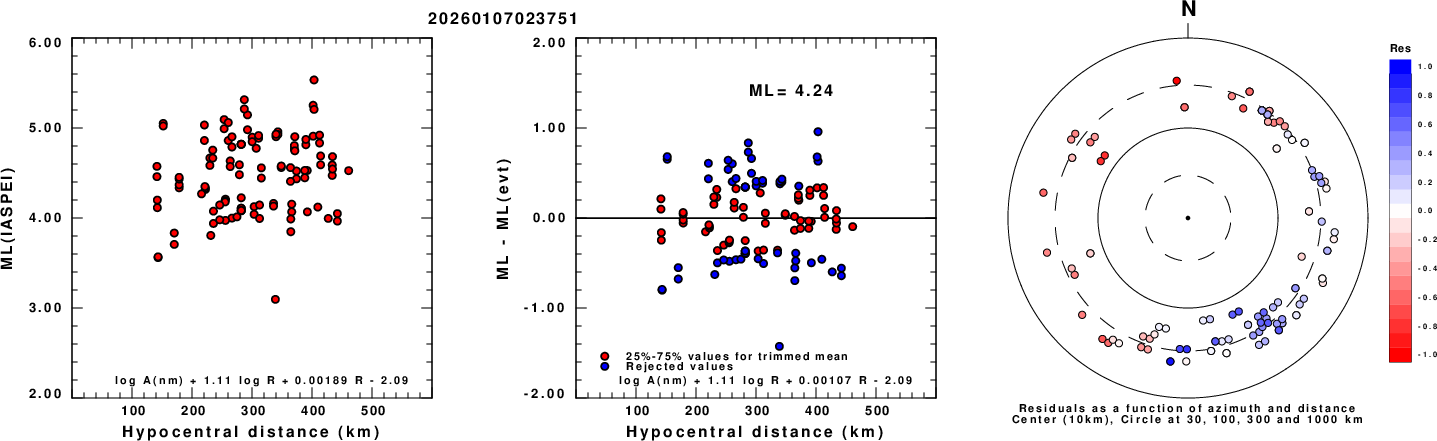
Left: ML computed using the IASPEI formula for Horizontal components. Center: ML residuals computed using a modified IASPEI formula that accounts for path specific attenuation; the values used for the trimmed mean are indicated. The ML relation used for each figure is given at the bottom of each plot.
Right: Residuals from new relation as a function of distance and azimuth.
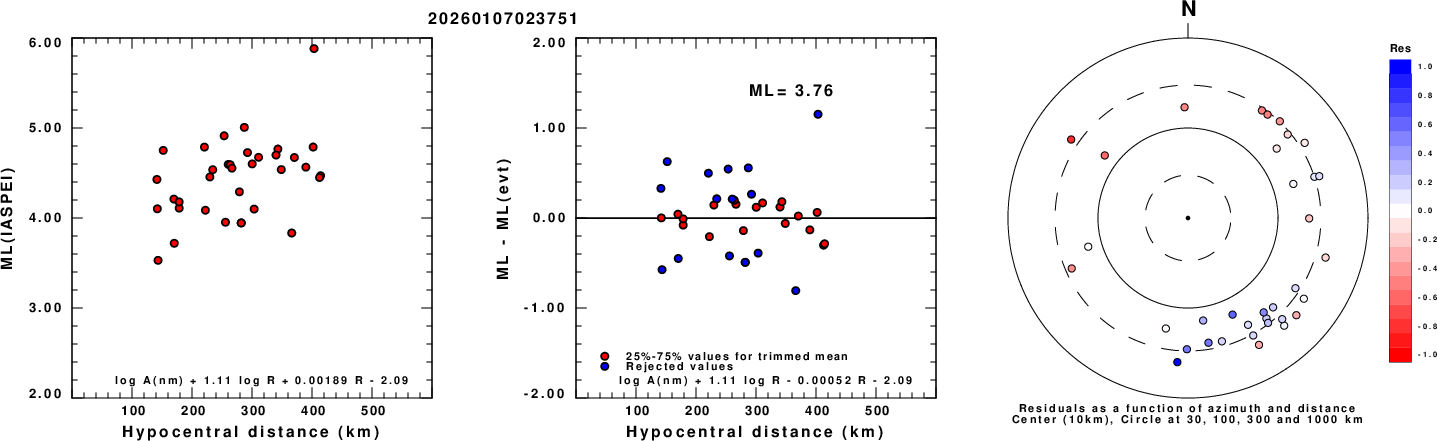
Left: ML computed using the IASPEI formula for Vertical components (research). Center: ML residuals computed using a modified IASPEI formula that accounts for path specific attenuation; the values used for the trimmed mean are indicated. The ML relation used for each figure is given at the bottom of each plot.
Right: Residuals from new relation as a function of distance and azimuth.
Context
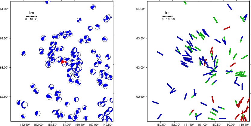
The left panel of the next figure presents the focal mechanism for this earthquake (red) in the context of other nearby events (blue) in the SLU Moment Tensor Catalog. The right panel shows the inferred direction of maximum compressive stress and the type of faulting (green is strike-slip, red is normal, blue is thrust; oblique is shown by a combination of colors). Thus context plot is useful for assessing the appropriateness of the moment tensor of this event.
Waveform Inversion using wvfgrd96
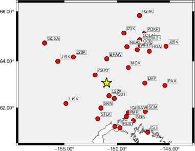
The focal mechanism was determined using broadband seismic waveforms. The location of the event (star) and the
stations used for (red) the waveform inversion are shown in the next figure.
|
|
Location of broadband stations used for waveform inversion
|
The program wvfgrd96 was used with good traces observed at short distance to determine the focal mechanism, depth and seismic moment. This technique requires a high quality signal and well determined velocity model for the Green's functions. To the extent that these are the quality data, this type of mechanism should be preferred over the radiation pattern technique which requires the separate step of defining the pressure and tension quadrants and the correct strike.
The observed and predicted traces are filtered using the following gsac commands:
cut o DIST/3.5 -40 o DIST/3.5 +50
rtr
taper w 0.1
hp c 0.03 n 3
lp c 0.08 n 3
The results of this grid search are as follow:
           DEPTH  STK   DIP  RAKE   MW    FIT
WVFGRD96   60.0    60    75    15   4.24 0.3185
WVFGRD96   62.0    55    70    15   4.25 0.3380
WVFGRD96   64.0    55    70    15   4.26 0.3546
WVFGRD96   66.0    55    70    15   4.27 0.3674
WVFGRD96   68.0    55    70    15   4.28 0.3766
WVFGRD96   70.0    55    70    15   4.29 0.3853
WVFGRD96   72.0    55    70    15   4.30 0.3929
WVFGRD96   74.0    55    70    15   4.30 0.4006
WVFGRD96   76.0    55    70    15   4.31 0.4077
WVFGRD96   78.0    55    70    15   4.31 0.4148
WVFGRD96   80.0    55    70    15   4.32 0.4224
WVFGRD96   82.0    55    70    15   4.32 0.4289
WVFGRD96   84.0    55    70    15   4.33 0.4347
WVFGRD96   86.0    60    70    20   4.33 0.4404
WVFGRD96   88.0    60    70    20   4.33 0.4466
WVFGRD96   90.0    60    70    20   4.34 0.4517
WVFGRD96   92.0    60    70    20   4.34 0.4564
WVFGRD96   94.0    55    75    20   4.35 0.4617
WVFGRD96   96.0    55    75    20   4.35 0.4669
WVFGRD96   98.0    55    75    20   4.36 0.4713
WVFGRD96  100.0    60    75    25   4.36 0.4757
WVFGRD96  102.0    60    75    25   4.37 0.4791
WVFGRD96  104.0    60    75    25   4.37 0.4837
WVFGRD96  106.0    60    75    25   4.37 0.4870
WVFGRD96  108.0    60    75    25   4.38 0.4897
WVFGRD96  110.0    60    75    25   4.38 0.4927
WVFGRD96  112.0    60    75    25   4.38 0.4953
WVFGRD96  114.0    60    75    25   4.39 0.4973
WVFGRD96  116.0    60    75    25   4.39 0.4988
WVFGRD96  118.0    60    75    30   4.39 0.5017
WVFGRD96  120.0    60    75    30   4.40 0.5025
WVFGRD96  122.0    60    75    30   4.40 0.5042
WVFGRD96  124.0    55    75    30   4.40 0.5058
WVFGRD96  126.0    55    75    30   4.40 0.5067
WVFGRD96  128.0    55    75    30   4.40 0.5076
WVFGRD96  130.0    55    75    30   4.41 0.5085
WVFGRD96  132.0    55    75    30   4.41 0.5079
WVFGRD96  134.0    55    75    30   4.41 0.5087
WVFGRD96  136.0    55    75    30   4.41 0.5083
WVFGRD96  138.0    55    75    30   4.41 0.5089
WVFGRD96  140.0    55    75    30   4.42 0.5080
WVFGRD96  142.0    55    75    30   4.42 0.5071
WVFGRD96  144.0    55    75    30   4.42 0.5064
WVFGRD96  146.0    55    75    30   4.42 0.5055
WVFGRD96  148.0    55    75    30   4.42 0.5049
WVFGRD96  150.0    60    70    30   4.42 0.5028
WVFGRD96  152.0    60    70    30   4.42 0.5026
WVFGRD96  154.0    60    70    30   4.43 0.5007
WVFGRD96  156.0    60    70    30   4.43 0.5002
WVFGRD96  158.0    60    70    30   4.43 0.4978
WVFGRD96  160.0    60    70    30   4.43 0.4971
WVFGRD96  162.0    60    70    30   4.43 0.4952
WVFGRD96  164.0    60    70    30   4.44 0.4938
WVFGRD96  166.0    60    70    30   4.44 0.4923
WVFGRD96  168.0    60    70    30   4.44 0.4919
WVFGRD96  170.0    60    70    30   4.44 0.4896
WVFGRD96  172.0    60    70    30   4.44 0.4854
WVFGRD96  174.0    60    70    30   4.44 0.4691
WVFGRD96  176.0    55    75    30   4.44 0.4448
WVFGRD96  178.0    55    75    35   4.43 0.4219
WVFGRD96  180.0    55    75    35   4.43 0.4005
WVFGRD96  182.0    55    75    35   4.42 0.3796
WVFGRD96  184.0    55    75    35   4.41 0.3575
WVFGRD96  186.0    55    75    35   4.41 0.3391
WVFGRD96  188.0    50    80    30   4.41 0.3195
The best solution is
WVFGRD96 138.0 55 75 30 4.41 0.5089
The mechanism corresponding to the best fit is
|
|
Figure 1. Waveform inversion focal mechanism
|
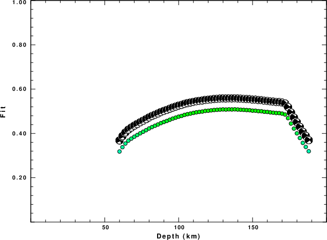
The best fit as a function of depth is given in the following figure:
|
|
Figure 2. Depth sensitivity for waveform mechanism
|
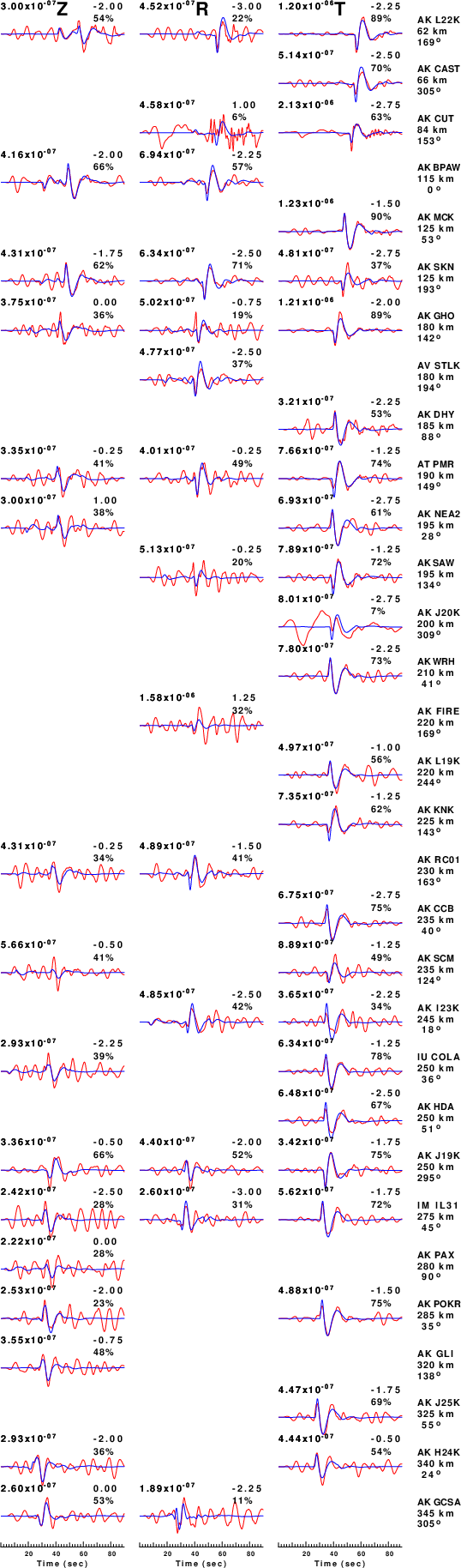
The comparison of the observed and predicted waveforms is given in the next figure. The red traces are the observed and the blue are the predicted.
Each observed-predicted component is plotted to the same scale and peak amplitudes are indicated by the numbers to the left of each trace. A pair of numbers is given in black at the right of each predicted traces. The upper number it the time shift required for maximum correlation between the observed and predicted traces. This time shift is required because the synthetics are not computed at exactly the same distance as the observed, the velocity model used in the predictions may not be perfect and the epicentral parameters may be be off.
A positive time shift indicates that the prediction is too fast and should be delayed to match the observed trace (shift to the right in this figure). A negative value indicates that the prediction is too slow. The lower number gives the percentage of variance reduction to characterize the individual goodness of fit (100% indicates a perfect fit).
The bandpass filter used in the processing and for the display was
cut o DIST/3.5 -40 o DIST/3.5 +50
rtr
taper w 0.1
hp c 0.03 n 3
lp c 0.08 n 3
|
|
Figure 3. Waveform comparison for selected depth. Red: observed; Blue - predicted. The time shift with respect to the model prediction is indicated. The percent of fit is also indicated. The time scale is relative to the first trace sample.
|
|
|
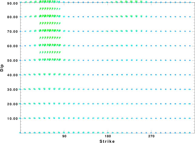
Focal mechanism sensitivity at the preferred depth. The red color indicates a very good fit to the waveforms.
Each solution is plotted as a vector at a given value of strike and dip with the angle of the vector representing the rake angle, measured, with respect to the upward vertical (N) in the figure.
|
A check on the assumed source location is possible by looking at the time shifts between the observed and predicted traces. The time shifts for waveform matching arise for several reasons:
- The origin time and epicentral distance are incorrect
- The velocity model used for the inversion is incorrect
- The velocity model used to define the P-arrival time is not the
same as the velocity model used for the waveform inversion
(assuming that the initial trace alignment is based on the
P arrival time)
Assuming only a mislocation, the time shifts are fit to a functional form:
Time_shift = A + B cos Azimuth + C Sin Azimuth
The time shifts for this inversion lead to the next figure:
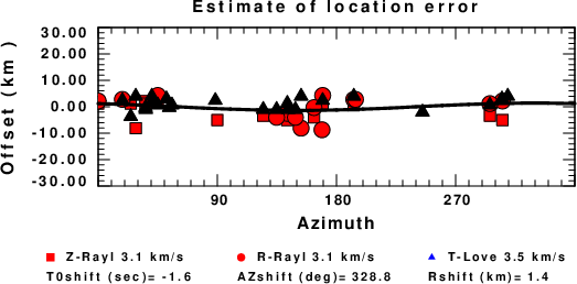
The derived shift in origin time and epicentral coordinates are given at the bottom of the figure.
Velocity Model
The WUS.model used for the waveform synthetic seismograms and for the surface wave eigenfunctions and dispersion is as follows
(The format is in the model96 format of Computer Programs in Seismology).
MODEL.01
Model after     8 iterations
ISOTROPIC
KGS
FLAT EARTH
1-D
CONSTANT VELOCITY
LINE08
LINE09
LINE10
LINE11
      H(KM)   VP(KM/S)   VS(KM/S) RHO(GM/CC)         QP         QS       ETAP       ETAS      FREFP      FREFS
     1.9000     3.4065     2.0089     2.2150  0.302E-02  0.679E-02   0.00       0.00       1.00       1.00
     6.1000     5.5445     3.2953     2.6089  0.349E-02  0.784E-02   0.00       0.00       1.00       1.00
    13.0000     6.2708     3.7396     2.7812  0.212E-02  0.476E-02   0.00       0.00       1.00       1.00
    19.0000     6.4075     3.7680     2.8223  0.111E-02  0.249E-02   0.00       0.00       1.00       1.00
     0.0000     7.9000     4.6200     3.2760  0.164E-10  0.370E-10   0.00       0.00       1.00       1.00
Last Changed Wed Jan 7 07:35:07 EST 2026