Location

Location ANSS

The ANSS event ID is ak025d59j5t5 and the event page is at https://earthquake.usgs.gov/earthquakes/eventpage/ak025d59j5t5/executive.

2025/10/13 16:51:16 60.198 -153.707 188.4 4.1 Alaska

Focal Mechanism

USGS/SLU Moment Tensor Solution ENS 2025/10/13 16:51:16.0 60.20 -153.71 188.4 4.1 Alaska Stations used: AK.BRLK AK.CAST AK.L17K AK.L19K AK.N15K AK.N18K AK.O14K AK.O18K AK.O19K AK.PPLA AK.SWD AV.RED II.KDAK Filtering commands used: cut o DIST/4.5 -10 o DIST/4.5 +60 rtr taper w 0.1 hp c 0.03 n 3 lp c 0.10 n 3 Best Fitting Double Couple Mo = 2.11e+22 dyne-cm Mw = 4.15 Z = 188 km Plane Strike Dip Rake NP1 355 75 45 NP2 250 47 159 Principal Axes: Axis Value Plunge Azimuth T 2.11e+22 42 223 N 0.00e+00 43 9 P -2.11e+22 17 117 Moment Tensor: (dyne-cm) Component Value Mxx 2.45e+21 Mxy 1.36e+22 Mxz -4.98e+21 Myy -9.92e+21 Myz -1.26e+22 Mzz 7.47e+21 ------######## -----------########### ---------------############# ----------------############## -------------------############### --------------######------------#### -----------###########---------------# ---------##############----------------- -------################----------------- ------###################----------------- -----####################----------------- ----#####################----------------- ---######################----------------- -#######################---------------- -######### ###########---------- --- ######### T ###########---------- P -- ######## ###########---------- - #####################------------- ###################----------- #################----------- ##############-------- #########----- Global CMT Convention Moment Tensor: R T P 7.47e+21 -4.98e+21 1.26e+22 -4.98e+21 2.45e+21 -1.36e+22 1.26e+22 -1.36e+22 -9.92e+21 Details of the solution is found at http://www.eas.slu.edu/eqc/eqc_mt/MECH.NA/20251013165116/index.html

Preferred Solution

The preferred solution from an analysis of the surface-wave spectral amplitude radiation pattern, waveform inversion or first motion observations is

      STK = 355
      DIP = 75
     RAKE = 45
       MW = 4.15
       HS = 188.0

The NDK file is 20251013165116.ndk The waveform inversion is preferred.

Magnitudes

Given the availability of digital waveforms for determination of the moment tensor, this section documents the added processing leading to mLg, if appropriate to the region, and M_L by application of the respective IASPEI formulae. As a research study, the linear distance term of the IASPEI formula for M_L is adjusted to remove a linear distance trend in residuals to give a regionally defined M_L. The defined M_L uses horizontal component recordings, but the same procedure is applied to the vertical components since there may be some interest in vertical component ground motions. Residual plots versus distance may indicate interesting features of ground motion scaling in some distance ranges. A residual plot of the regionalized magnitude is given as a function of distance and azimuth, since data sets may transcend different wave propagation provinces.

ML Magnitude

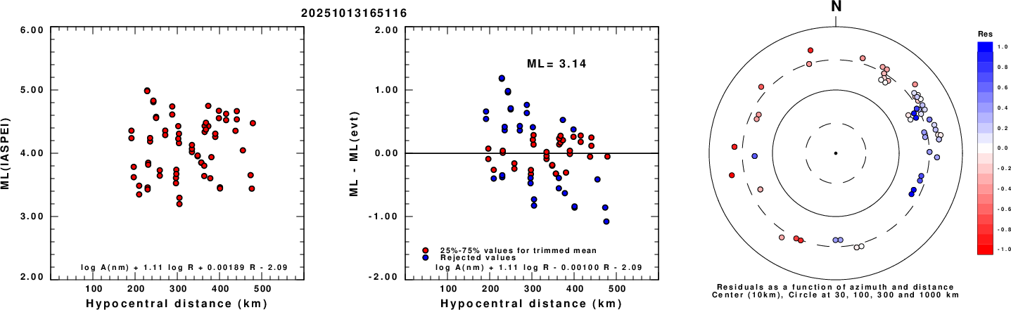
Left: ML computed using the IASPEI formula for Horizontal components. Center: ML residuals computed using a modified IASPEI formula that accounts for path specific attenuation; the values used for the trimmed mean are indicated. The ML relation used for each figure is given at the bottom of each plot. Right: Residuals from new relation as a function of distance and azimuth.

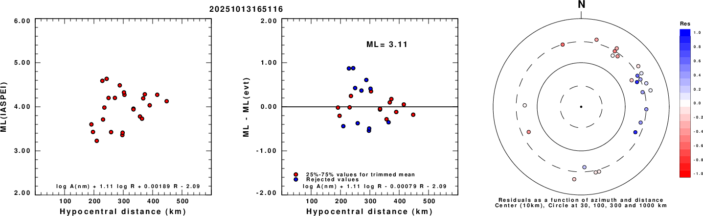
Left: ML computed using the IASPEI formula for Vertical components (research). Center: ML residuals computed using a modified IASPEI formula that accounts for path specific attenuation; the values used for the trimmed mean are indicated. The ML relation used for each figure is given at the bottom of each plot. Right: Residuals from new relation as a function of distance and azimuth.

Context

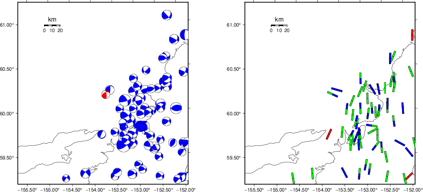
The left panel of the next figure presents the focal mechanism for this earthquake (red) in the context of other nearby events (blue) in the SLU Moment Tensor Catalog. The right panel shows the inferred direction of maximum compressive stress and the type of faulting (green is strike-slip, red is normal, blue is thrust; oblique is shown by a combination of colors). Thus context plot is useful for assessing the appropriateness of the moment tensor of this event.

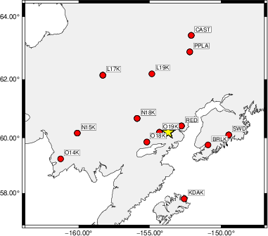
Waveform Inversion using wvfgrd96

The focal mechanism was determined using broadband seismic waveforms. The location of the event (star) and the stations used for (red) the waveform inversion are shown in the next figure.

Location of broadband stations used for waveform inversion

The program wvfgrd96 was used with good traces observed at short distance to determine the focal mechanism, depth and seismic moment. This technique requires a high quality signal and well determined velocity model for the Green's functions. To the extent that these are the quality data, this type of mechanism should be preferred over the radiation pattern technique which requires the separate step of defining the pressure and tension quadrants and the correct strike.

The observed and predicted traces are filtered using the following gsac commands:

cut o DIST/4.5 -10 o DIST/4.5 +60
rtr
taper w 0.1
hp c 0.03 n 3 
lp c 0.10 n 3

The results of this grid search are as follow:

           DEPTH  STK   DIP  RAKE   MW    FIT
WVFGRD96  120.0    35    45    50   3.99 0.2005
WVFGRD96  122.0    35    45    50   4.00 0.2040
WVFGRD96  124.0    20    55    45   4.00 0.2148
WVFGRD96  126.0    20    55    50   4.00 0.2295
WVFGRD96  128.0    15    60    45   4.01 0.2474
WVFGRD96  130.0    15    60    50   4.04 0.3033
WVFGRD96  132.0     5    65    50   4.05 0.3593
WVFGRD96  134.0     5    65    55   4.07 0.4062
WVFGRD96  136.0     0    70    50   4.08 0.4501
WVFGRD96  138.0    -5    75    45   4.09 0.4808
WVFGRD96  140.0    -5    75    45   4.10 0.5030
WVFGRD96  142.0    -5    75    45   4.11 0.5121
WVFGRD96  144.0    -5    75    45   4.11 0.5143
WVFGRD96  146.0   355    75    45   4.11 0.5175
WVFGRD96  148.0   355    75    45   4.11 0.5189
WVFGRD96  150.0   355    75    45   4.12 0.5216
WVFGRD96  152.0   355    75    45   4.12 0.5239
WVFGRD96  154.0   355    75    45   4.12 0.5250
WVFGRD96  156.0   355    75    45   4.12 0.5256
WVFGRD96  158.0   355    75    45   4.12 0.5268
WVFGRD96  160.0   355    75    45   4.12 0.5276
WVFGRD96  162.0   355    75    45   4.13 0.5265
WVFGRD96  164.0    -5    75    45   4.13 0.5289
WVFGRD96  166.0   355    75    45   4.13 0.5295
WVFGRD96  168.0   355    75    45   4.13 0.5291
WVFGRD96  170.0    -5    75    45   4.13 0.5306
WVFGRD96  172.0    -5    75    45   4.13 0.5310
WVFGRD96  174.0    -5    75    45   4.13 0.5303
WVFGRD96  176.0    -5    75    45   4.14 0.5311
WVFGRD96  178.0   355    75    45   4.14 0.5310
WVFGRD96  180.0   355    75    45   4.14 0.5310
WVFGRD96  182.0   355    75    45   4.14 0.5318
WVFGRD96  184.0   355    75    45   4.14 0.5319
WVFGRD96  186.0   355    75    45   4.14 0.5311
WVFGRD96  188.0   355    75    45   4.15 0.5321
WVFGRD96  190.0   355    75    45   4.15 0.5312
WVFGRD96  192.0   355    75    45   4.15 0.5314
WVFGRD96  194.0   355    75    45   4.15 0.5300
WVFGRD96  196.0   355    75    45   4.15 0.5310
WVFGRD96  198.0   355    75    45   4.15 0.5293

The best solution is

WVFGRD96  188.0   355    75    45   4.15 0.5321

The mechanism corresponding to the best fit is

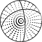
Figure 1. Waveform inversion focal mechanism

The best fit as a function of depth is given in the following figure:

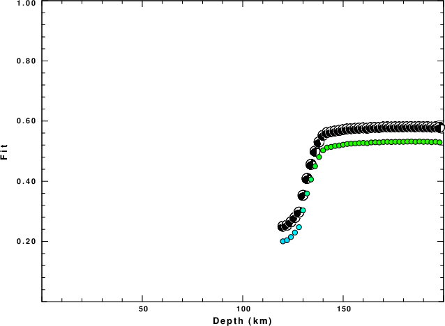
Figure 2. Depth sensitivity for waveform mechanism

The comparison of the observed and predicted waveforms is given in the next figure. The red traces are the observed and the blue are the predicted. Each observed-predicted component is plotted to the same scale and peak amplitudes are indicated by the numbers to the left of each trace. A pair of numbers is given in black at the right of each predicted traces. The upper number it the time shift required for maximum correlation between the observed and predicted traces. This time shift is required because the synthetics are not computed at exactly the same distance as the observed, the velocity model used in the predictions may not be perfect and the epicentral parameters may be be off. A positive time shift indicates that the prediction is too fast and should be delayed to match the observed trace (shift to the right in this figure). A negative value indicates that the prediction is too slow. The lower number gives the percentage of variance reduction to characterize the individual goodness of fit (100% indicates a perfect fit).

The bandpass filter used in the processing and for the display was

cut o DIST/4.5 -10 o DIST/4.5 +60
rtr
taper w 0.1
hp c 0.03 n 3 
lp c 0.10 n 3

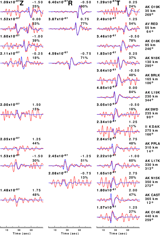
Figure 3. Waveform comparison for selected depth. Red: observed; Blue - predicted. The time shift with respect to the model prediction is indicated. The percent of fit is also indicated. The time scale is relative to the first trace sample.

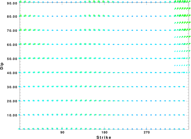
Focal mechanism sensitivity at the preferred depth. The red color indicates a very good fit to the waveforms. Each solution is plotted as a vector at a given value of strike and dip with the angle of the vector representing the rake angle, measured, with respect to the upward vertical (N) in the figure.

A check on the assumed source location is possible by looking at the time shifts between the observed and predicted traces. The time shifts for waveform matching arise for several reasons:

The origin time and epicentral distance are incorrect
The velocity model used for the inversion is incorrect
The velocity model used to define the P-arrival time is not the same as the velocity model used for the waveform inversion (assuming that the initial trace alignment is based on the P arrival time)

Assuming only a mislocation, the time shifts are fit to a functional form:

 Time_shift = A + B cos Azimuth + C Sin Azimuth

The time shifts for this inversion lead to the next figure:

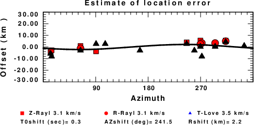
The derived shift in origin time and epicentral coordinates are given at the bottom of the figure.

Velocity Model

The WUS.model used for the waveform synthetic seismograms and for the surface wave eigenfunctions and dispersion is as follows (The format is in the model96 format of Computer Programs in Seismology).

MODEL.01
Model after     8 iterations
ISOTROPIC
KGS
FLAT EARTH
1-D
CONSTANT VELOCITY
LINE08
LINE09
LINE10
LINE11
      H(KM)   VP(KM/S)   VS(KM/S) RHO(GM/CC)         QP         QS       ETAP       ETAS      FREFP      FREFS
     1.9000     3.4065     2.0089     2.2150  0.302E-02  0.679E-02   0.00       0.00       1.00       1.00    
     6.1000     5.5445     3.2953     2.6089  0.349E-02  0.784E-02   0.00       0.00       1.00       1.00    
    13.0000     6.2708     3.7396     2.7812  0.212E-02  0.476E-02   0.00       0.00       1.00       1.00    
    19.0000     6.4075     3.7680     2.8223  0.111E-02  0.249E-02   0.00       0.00       1.00       1.00    
     0.0000     7.9000     4.6200     3.2760  0.164E-10  0.370E-10   0.00       0.00       1.00       1.00

Last Changed Mon Oct 13 14:04:03 CDT 2025