Location
Location ANSS
The ANSS event ID is uu80117176 and the event page is at
https://earthquake.usgs.gov/earthquakes/eventpage/uu80117176/executive.
2025/09/10 23:57:47 40.475 -109.696 69.4 4.1 Utah
Focal Mechanism
 USGS/SLU Moment Tensor Solution
 ENS  2025/09/10 23:57:47.0  40.47 -109.70  69.4 4.1 Utah

 Stations used:
   C0.HAYD C0.MOFF N4.K22A N4.O20A UU.BRPU UU.BSUT UU.CTU
   UU.GAWY UU.HDUT UU.HLJ UU.LIUT UU.MCU UU.SRU UU.SVWY UU.TMU

 Filtering commands used:
   cut o DIST/3.3 -30 o DIST/3.3 +30
   rtr
   taper w 0.1
   hp c 0.05 n 3
   lp c 0.15 n 3

 Best Fitting Double Couple
  Mo = 1.66e+22 dyne-cm
  Mw = 4.08
  Z  = 64 km
  Plane   Strike  Dip  Rake
   NP1      110    65    40
   NP2        0    54   149
  Principal Axes:
   Axis    Value   Plunge  Azimuth
    T   1.66e+22     45     330
    N   0.00e+00     44     137
    P  -1.66e+22      6     233

 Moment Tensor: (dyne-cm)
    Component   Value
       Mxx     1.90e+20
       Mxy    -1.15e+22
       Mxz     8.28e+21
       Myy    -8.36e+21
       Myz    -2.70e+21
       Mzz     8.17e+21


                     #########-----
                 ###############-------
              ###################---------
             #####################---------
           ##########   ###########----------
          ########### T ###########-----------
         ############   ############-----------
        -###########################------------
        --###########################-----------
       -----#########################------------
       -------#######################------------
       ---------#####################------------
       ------------##################------------
        ---------------##############-----------
        -------------------#########------------
         ----------------------------------####
          -   ---------------------###########
            P ---------------------##########
              --------------------#########
              -------------------#########
                 --------------########
                     ---------#####


 Global CMT Convention Moment Tensor:
      R          T          P
  8.17e+21   8.28e+21   2.70e+21
  8.28e+21   1.90e+20   1.15e+22
  2.70e+21   1.15e+22  -8.36e+21


Details of the solution is found at

http://www.eas.slu.edu/eqc/eqc_mt/MECH.NA/20250910235747/index.html
|
Preferred Solution
The preferred solution from an analysis of the surface-wave spectral amplitude radiation pattern, waveform inversion or first motion observations is
      STK = 110
      DIP = 65
     RAKE = 40
       MW = 4.08
       HS = 64.0
The NDK file is 20250910235747.ndk
The waveform inversion is preferred.
Moment Tensor Comparison
The following compares this source inversion to those provided by others. The purpose is to look for major differences and also to note slight differences that might be inherent to the processing procedure. For completeness the USGS/SLU solution is repeated from above.
| SLU |
USGSMWR |
 USGS/SLU Moment Tensor Solution
 ENS  2025/09/10 23:57:47.0  40.47 -109.70  69.4 4.1 Utah

 Stations used:
   C0.HAYD C0.MOFF N4.K22A N4.O20A UU.BRPU UU.BSUT UU.CTU
   UU.GAWY UU.HDUT UU.HLJ UU.LIUT UU.MCU UU.SRU UU.SVWY UU.TMU

 Filtering commands used:
   cut o DIST/3.3 -30 o DIST/3.3 +30
   rtr
   taper w 0.1
   hp c 0.05 n 3
   lp c 0.15 n 3

 Best Fitting Double Couple
  Mo = 1.66e+22 dyne-cm
  Mw = 4.08
  Z  = 64 km
  Plane   Strike  Dip  Rake
   NP1      110    65    40
   NP2        0    54   149
  Principal Axes:
   Axis    Value   Plunge  Azimuth
    T   1.66e+22     45     330
    N   0.00e+00     44     137
    P  -1.66e+22      6     233

 Moment Tensor: (dyne-cm)
    Component   Value
       Mxx     1.90e+20
       Mxy    -1.15e+22
       Mxz     8.28e+21
       Myy    -8.36e+21
       Myz    -2.70e+21
       Mzz     8.17e+21


                     #########-----
                 ###############-------
              ###################---------
             #####################---------
           ##########   ###########----------
          ########### T ###########-----------
         ############   ############-----------
        -###########################------------
        --###########################-----------
       -----#########################------------
       -------#######################------------
       ---------#####################------------
       ------------##################------------
        ---------------##############-----------
        -------------------#########------------
         ----------------------------------####
          -   ---------------------###########
            P ---------------------##########
              --------------------#########
              -------------------#########
                 --------------########
                     ---------#####


 Global CMT Convention Moment Tensor:
      R          T          P
  8.17e+21   8.28e+21   2.70e+21
  8.28e+21   1.90e+20   1.15e+22
  2.70e+21   1.15e+22  -8.36e+21


Details of the solution is found at

http://www.eas.slu.edu/eqc/eqc_mt/MECH.NA/20250910235747/index.html
|
Regional Moment Tensor (Mwr)
Moment 1.842e+15 N-m
Magnitude 4.11 Mwr
Depth 67.0 km
Percent DC 88%
Half Duration -
Catalog US
Data Source US
Contributor US
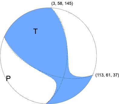
Nodal Planes
Plane Strike Dip Rake
NP1 3 58 145
NP2 113 61 37
Principal Axes
Axis Value Plunge Azimuth
T 1.784e+15 46 330
N 0.112e+15 44 146
P -1.896e+15 2 238
|
Magnitudes
Given the availability of digital waveforms for determination of the moment tensor, this section documents the added processing leading to mLg, if appropriate to the region, and ML by application of the respective IASPEI formulae. As a research study, the linear distance term of the IASPEI formula
for ML is adjusted to remove a linear distance trend in residuals to give a regionally defined ML. The defined ML uses horizontal component recordings, but the same procedure is applied to the vertical components since there may be some interest in vertical component ground motions. Residual plots versus distance may indicate interesting features of ground motion scaling in some distance ranges. A residual plot of the regionalized magnitude is given as a function of distance and azimuth, since data sets may transcend different wave propagation provinces.
ML Magnitude
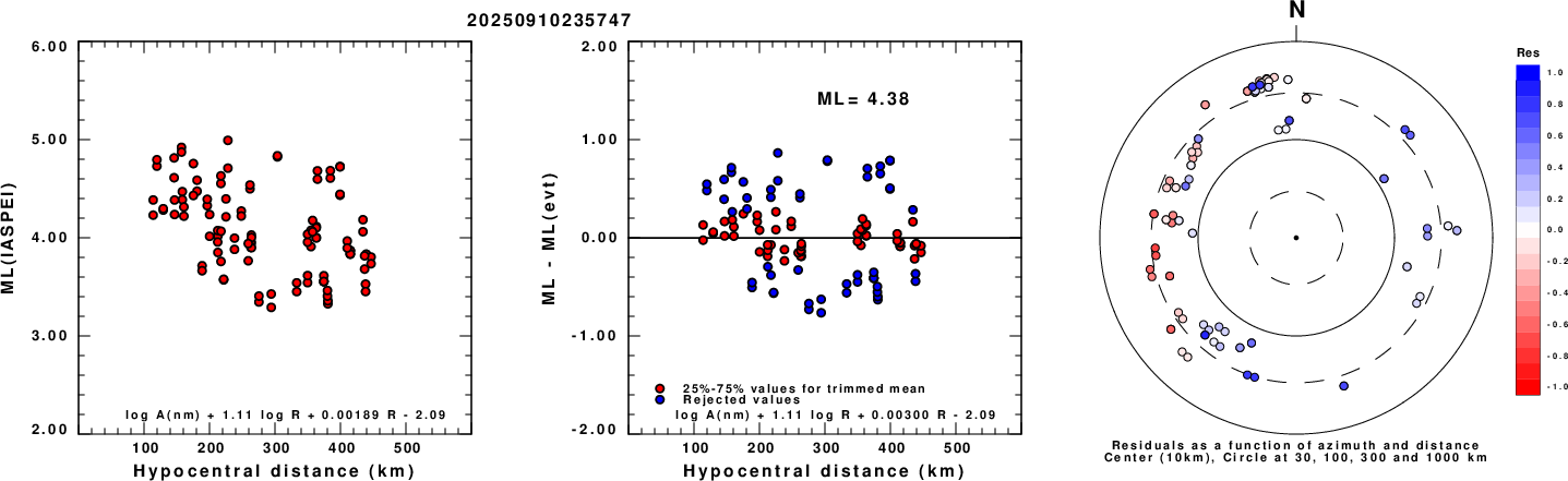
Left: ML computed using the IASPEI formula for Horizontal components. Center: ML residuals computed using a modified IASPEI formula that accounts for path specific attenuation; the values used for the trimmed mean are indicated. The ML relation used for each figure is given at the bottom of each plot.
Right: Residuals from new relation as a function of distance and azimuth.
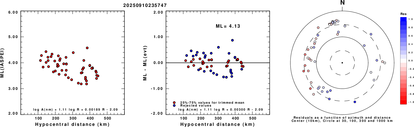
Left: ML computed using the IASPEI formula for Vertical components (research). Center: ML residuals computed using a modified IASPEI formula that accounts for path specific attenuation; the values used for the trimmed mean are indicated. The ML relation used for each figure is given at the bottom of each plot.
Right: Residuals from new relation as a function of distance and azimuth.
Context
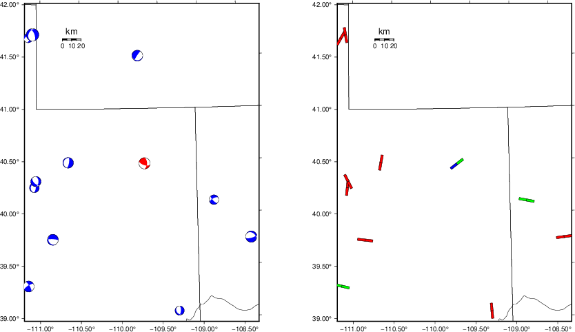
The left panel of the next figure presents the focal mechanism for this earthquake (red) in the context of other nearby events (blue) in the SLU Moment Tensor Catalog. The right panel shows the inferred direction of maximum compressive stress and the type of faulting (green is strike-slip, red is normal, blue is thrust; oblique is shown by a combination of colors). Thus context plot is useful for assessing the appropriateness of the moment tensor of this event.
Waveform Inversion using wvfgrd96
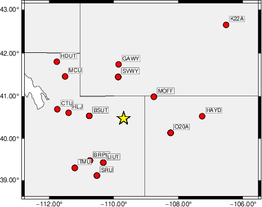
The focal mechanism was determined using broadband seismic waveforms. The location of the event (star) and the
stations used for (red) the waveform inversion are shown in the next figure.
|
|
Location of broadband stations used for waveform inversion
|
The program wvfgrd96 was used with good traces observed at short distance to determine the focal mechanism, depth and seismic moment. This technique requires a high quality signal and well determined velocity model for the Green's functions. To the extent that these are the quality data, this type of mechanism should be preferred over the radiation pattern technique which requires the separate step of defining the pressure and tension quadrants and the correct strike.
The observed and predicted traces are filtered using the following gsac commands:
cut o DIST/3.3 -30 o DIST/3.3 +30
rtr
taper w 0.1
hp c 0.05 n 3
lp c 0.15 n 3
The results of this grid search are as follow:
           DEPTH  STK   DIP  RAKE   MW    FIT
WVFGRD96    2.0   150    50   -85   3.21 0.1881
WVFGRD96    4.0   350    65   -50   3.25 0.2211
WVFGRD96    6.0   350    60   -45   3.31 0.2406
WVFGRD96    8.0   350    65   -45   3.42 0.2522
WVFGRD96   10.0   190    75    35   3.46 0.2470
WVFGRD96   12.0   270    60   -25   3.52 0.2362
WVFGRD96   14.0     5    60   -30   3.56 0.2260
WVFGRD96   16.0   285    65    25   3.60 0.2282
WVFGRD96   18.0   285    60    30   3.64 0.2407
WVFGRD96   20.0   285    60    30   3.68 0.2636
WVFGRD96   22.0   285    60    35   3.71 0.2784
WVFGRD96   24.0   285    65    40   3.72 0.2950
WVFGRD96   26.0   285    65    35   3.74 0.3121
WVFGRD96   28.0   285    65    35   3.74 0.3171
WVFGRD96   30.0   290    65    35   3.75 0.3166
WVFGRD96   32.0   290    55    40   3.76 0.3364
WVFGRD96   34.0   120    65    35   3.80 0.3665
WVFGRD96   36.0   115    70    35   3.81 0.3946
WVFGRD96   38.0   115    70    35   3.84 0.4136
WVFGRD96   40.0   295    55    45   3.90 0.4279
WVFGRD96   42.0   290    60    40   3.94 0.4345
WVFGRD96   44.0   115    70    35   3.98 0.4375
WVFGRD96   46.0   115    65    35   4.00 0.4377
WVFGRD96   48.0   115    55    35   4.02 0.4530
WVFGRD96   50.0   115    60    35   4.03 0.4841
WVFGRD96   52.0   115    60    35   4.05 0.5126
WVFGRD96   54.0   115    60    40   4.06 0.5391
WVFGRD96   56.0   115    60    40   4.07 0.5611
WVFGRD96   58.0   115    60    40   4.07 0.5739
WVFGRD96   60.0   115    60    40   4.08 0.5876
WVFGRD96   62.0   110    65    40   4.08 0.5928
WVFGRD96   64.0   110    65    40   4.08 0.5964
WVFGRD96   66.0   110    65    40   4.08 0.5949
WVFGRD96   68.0   110    65    40   4.08 0.5926
WVFGRD96   70.0   110    65    40   4.08 0.5874
WVFGRD96   72.0   110    65    40   4.08 0.5798
WVFGRD96   74.0   110    65    40   4.08 0.5707
WVFGRD96   76.0   110    65    40   4.08 0.5626
WVFGRD96   78.0   105    65    40   4.08 0.5551
WVFGRD96   80.0   105    65    40   4.08 0.5462
WVFGRD96   82.0   105    65    40   4.08 0.5354
WVFGRD96   84.0   105    65    35   4.08 0.5279
WVFGRD96   86.0   105    65    35   4.08 0.5199
WVFGRD96   88.0   105    65    35   4.08 0.5131
WVFGRD96   90.0   100    60    40   4.09 0.5084
WVFGRD96   92.0   100    60    40   4.09 0.5038
WVFGRD96   94.0   100    60    40   4.09 0.4995
WVFGRD96   96.0   100    60    40   4.09 0.4947
WVFGRD96   98.0   100    60    40   4.10 0.4899
The best solution is
WVFGRD96 64.0 110 65 40 4.08 0.5964
The mechanism corresponding to the best fit is
|
|
Figure 1. Waveform inversion focal mechanism
|
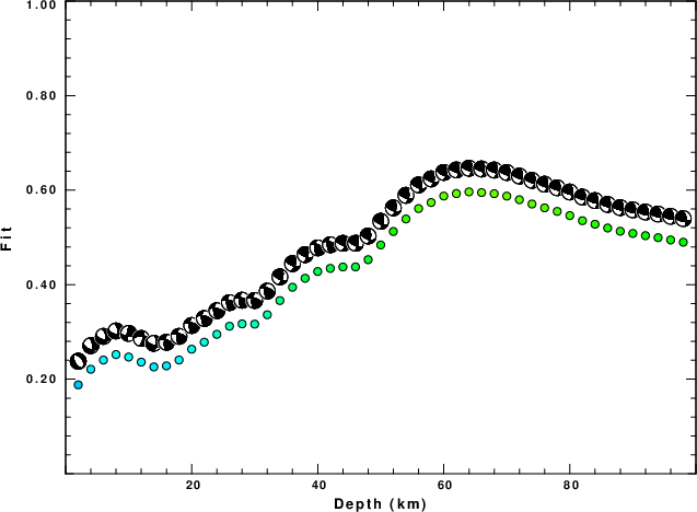
The best fit as a function of depth is given in the following figure:
|
|
Figure 2. Depth sensitivity for waveform mechanism
|
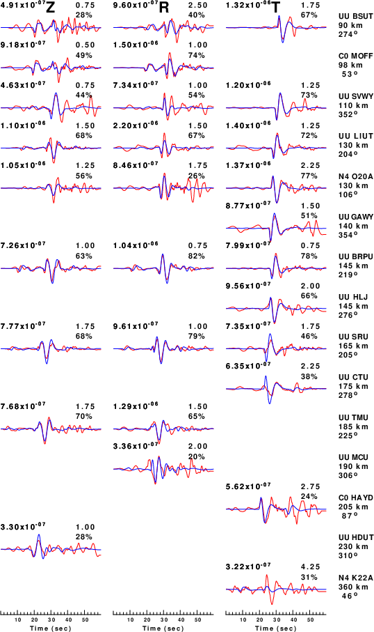
The comparison of the observed and predicted waveforms is given in the next figure. The red traces are the observed and the blue are the predicted.
Each observed-predicted component is plotted to the same scale and peak amplitudes are indicated by the numbers to the left of each trace. A pair of numbers is given in black at the right of each predicted traces. The upper number it the time shift required for maximum correlation between the observed and predicted traces. This time shift is required because the synthetics are not computed at exactly the same distance as the observed, the velocity model used in the predictions may not be perfect and the epicentral parameters may be be off.
A positive time shift indicates that the prediction is too fast and should be delayed to match the observed trace (shift to the right in this figure). A negative value indicates that the prediction is too slow. The lower number gives the percentage of variance reduction to characterize the individual goodness of fit (100% indicates a perfect fit).
The bandpass filter used in the processing and for the display was
cut o DIST/3.3 -30 o DIST/3.3 +30
rtr
taper w 0.1
hp c 0.05 n 3
lp c 0.15 n 3
|
|
Figure 3. Waveform comparison for selected depth. Red: observed; Blue - predicted. The time shift with respect to the model prediction is indicated. The percent of fit is also indicated. The time scale is relative to the first trace sample.
|
|
|
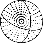
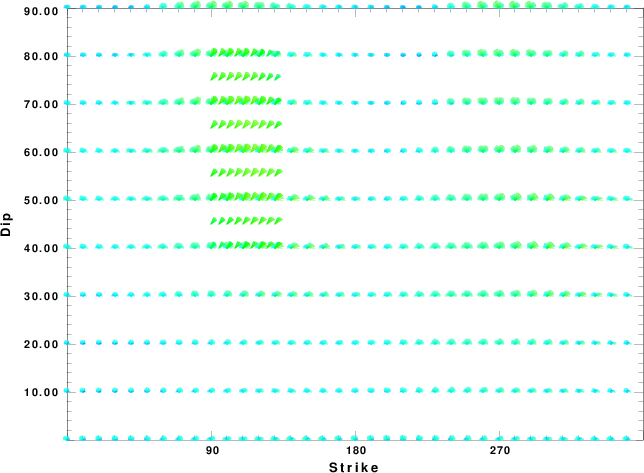
Focal mechanism sensitivity at the preferred depth. The red color indicates a very good fit to the waveforms.
Each solution is plotted as a vector at a given value of strike and dip with the angle of the vector representing the rake angle, measured, with respect to the upward vertical (N) in the figure.
|
A check on the assumed source location is possible by looking at the time shifts between the observed and predicted traces. The time shifts for waveform matching arise for several reasons:
- The origin time and epicentral distance are incorrect
- The velocity model used for the inversion is incorrect
- The velocity model used to define the P-arrival time is not the
same as the velocity model used for the waveform inversion
(assuming that the initial trace alignment is based on the
P arrival time)
Assuming only a mislocation, the time shifts are fit to a functional form:
Time_shift = A + B cos Azimuth + C Sin Azimuth
The time shifts for this inversion lead to the next figure:
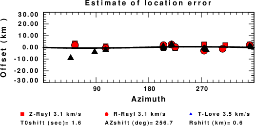
The derived shift in origin time and epicentral coordinates are given at the bottom of the figure.
Velocity Model
The WUS.model used for the waveform synthetic seismograms and for the surface wave eigenfunctions and dispersion is as follows
(The format is in the model96 format of Computer Programs in Seismology).
MODEL.01
Model after     8 iterations
ISOTROPIC
KGS
FLAT EARTH
1-D
CONSTANT VELOCITY
LINE08
LINE09
LINE10
LINE11
      H(KM)   VP(KM/S)   VS(KM/S) RHO(GM/CC)         QP         QS       ETAP       ETAS      FREFP      FREFS
     1.9000     3.4065     2.0089     2.2150  0.302E-02  0.679E-02   0.00       0.00       1.00       1.00
     6.1000     5.5445     3.2953     2.6089  0.349E-02  0.784E-02   0.00       0.00       1.00       1.00
    13.0000     6.2708     3.7396     2.7812  0.212E-02  0.476E-02   0.00       0.00       1.00       1.00
    19.0000     6.4075     3.7680     2.8223  0.111E-02  0.249E-02   0.00       0.00       1.00       1.00
     0.0000     7.9000     4.6200     3.2760  0.164E-10  0.370E-10   0.00       0.00       1.00       1.00
Last Changed Wed Sep 10 20:18:45 CDT 2025