Location
Location ANSS
The ANSS event ID is ak025a0u3q2q and the event page is at
https://earthquake.usgs.gov/earthquakes/eventpage/ak025a0u3q2q/executive.
2025/08/06 18:38:57 62.447 -151.216 84.4 4.6 Alaska
Focal Mechanism
 USGS/SLU Moment Tensor Solution
 ENS  2025/08/06 18:38:57.0  62.45 -151.22  84.4 4.6 Alaska

 Stations used:
   AK.BAE AK.BPAW AK.BRLK AK.CAST AK.DHY AK.FID AK.GHO AK.J19K
   AK.J20K AK.KNK AK.KTH AK.L19K AK.L22K AK.M20K AK.MCK AK.MLY
   AK.PAX AK.PPLA AK.PWL AK.RC01 AK.RND AK.SAW AK.SCM AK.SKN
   AK.SLK AK.SSN AK.WAT6 AT.PMR AT.TTA AV.RED AV.SPCL AV.STLK

 Filtering commands used:
   cut o DIST/3.5 -40 o DIST/3.5 +50
   rtr
   taper w 0.1
   hp c 0.03 n 3
   lp c 0.10 n 3

 Best Fitting Double Couple
  Mo = 1.23e+23 dyne-cm
  Mw = 4.66
  Z  = 96 km
  Plane   Strike  Dip  Rake
   NP1       45    90    70
   NP2      315    20   180
  Principal Axes:
   Axis    Value   Plunge  Azimuth
    T   1.23e+23     42     296
    N   0.00e+00     20      45
    P  -1.23e+23     42     154

 Moment Tensor: (dyne-cm)
    Component   Value
       Mxx    -4.21e+22
       Mxy    -6.89e+15
       Mxz     8.17e+22
       Myy     4.21e+22
       Myz    -8.17e+22
       Mzz    -1.01e+16


                     --------------
                 ---##########---------
              -####################-------
             #########################----#
           ##################################
          ############################---#####
         ###########################-------####
        ########   ###############----------####
        ######## T ##############------------###
       #########   ############--------------####
       ######################-----------------###
       ####################-------------------###
       ##################---------------------###
        ###############-----------------------##
        ##############------------------------##
         ###########------------   -----------#
          ########-------------- P ----------#
           #####----------------   ---------#
             #-----------------------------
              ----------------------------
                 ----------------------
                     --------------


 Global CMT Convention Moment Tensor:
      R          T          P
 -1.01e+16   8.17e+22   8.17e+22
  8.17e+22  -4.21e+22   6.89e+15
  8.17e+22   6.89e+15   4.21e+22


Details of the solution is found at

http://www.eas.slu.edu/eqc/eqc_mt/MECH.NA/20250806183857/index.html
|
Preferred Solution
The preferred solution from an analysis of the surface-wave spectral amplitude radiation pattern, waveform inversion or first motion observations is
      STK = 45
      DIP = 90
     RAKE = 70
       MW = 4.66
       HS = 96.0
The NDK file is 20250806183857.ndk
The waveform inversion is preferred.
Magnitudes
Given the availability of digital waveforms for determination of the moment tensor, this section documents the added processing leading to mLg, if appropriate to the region, and ML by application of the respective IASPEI formulae. As a research study, the linear distance term of the IASPEI formula
for ML is adjusted to remove a linear distance trend in residuals to give a regionally defined ML. The defined ML uses horizontal component recordings, but the same procedure is applied to the vertical components since there may be some interest in vertical component ground motions. Residual plots versus distance may indicate interesting features of ground motion scaling in some distance ranges. A residual plot of the regionalized magnitude is given as a function of distance and azimuth, since data sets may transcend different wave propagation provinces.
ML Magnitude
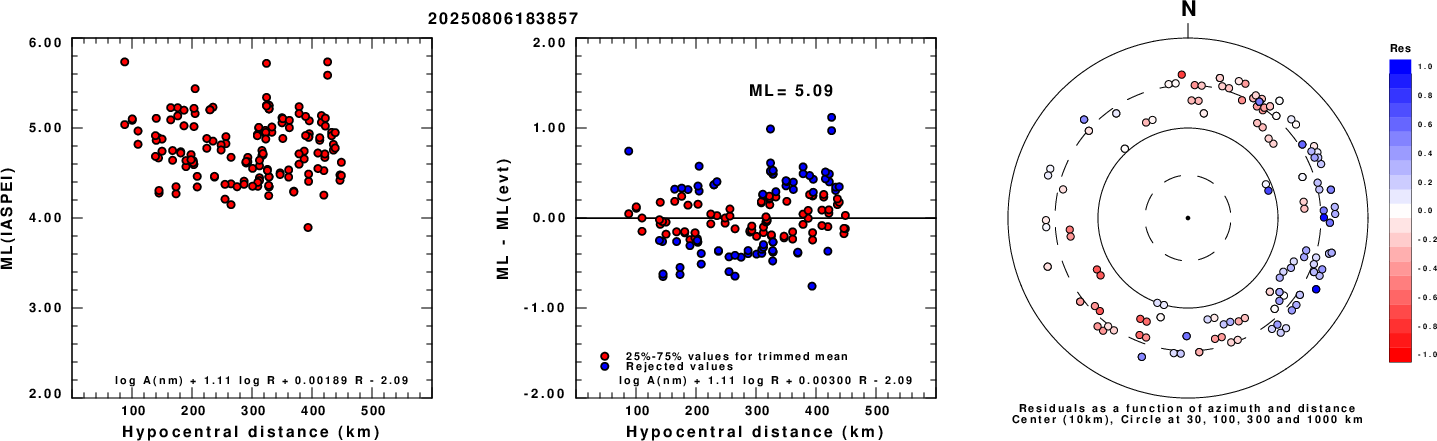
Left: ML computed using the IASPEI formula for Horizontal components. Center: ML residuals computed using a modified IASPEI formula that accounts for path specific attenuation; the values used for the trimmed mean are indicated. The ML relation used for each figure is given at the bottom of each plot.
Right: Residuals from new relation as a function of distance and azimuth.
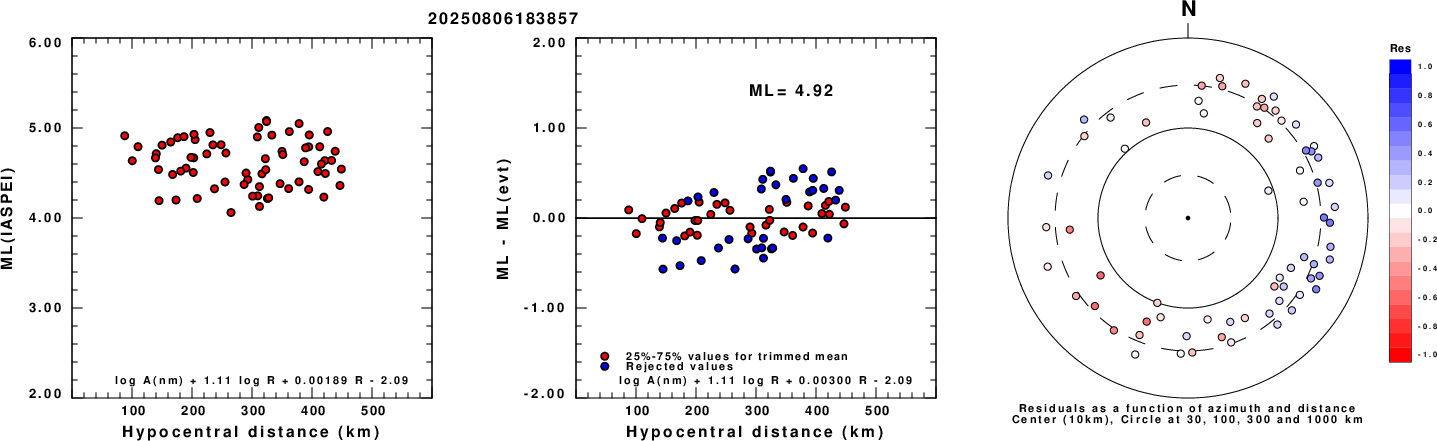
Left: ML computed using the IASPEI formula for Vertical components (research). Center: ML residuals computed using a modified IASPEI formula that accounts for path specific attenuation; the values used for the trimmed mean are indicated. The ML relation used for each figure is given at the bottom of each plot.
Right: Residuals from new relation as a function of distance and azimuth.
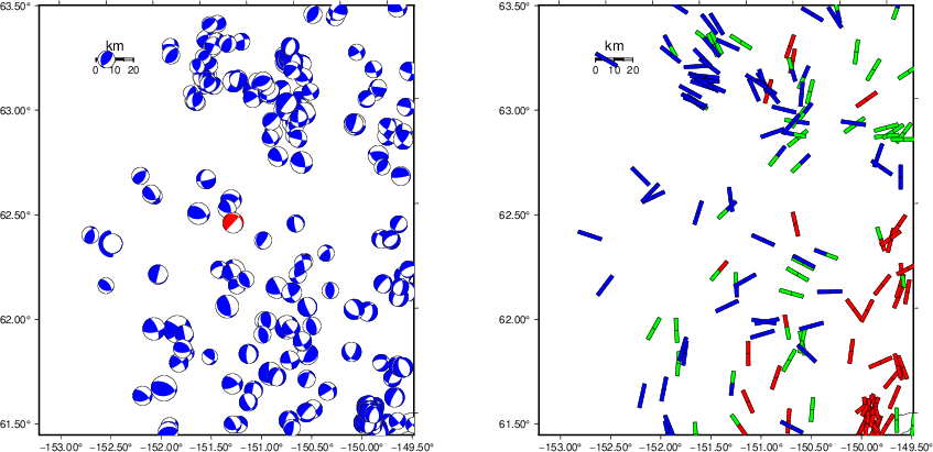
Context
The left panel of the next figure presents the focal mechanism for this earthquake (red) in the context of other nearby events (blue) in the SLU Moment Tensor Catalog. The right panel shows the inferred direction of maximum compressive stress and the type of faulting (green is strike-slip, red is normal, blue is thrust; oblique is shown by a combination of colors). Thus context plot is useful for assessing the appropriateness of the moment tensor of this event.
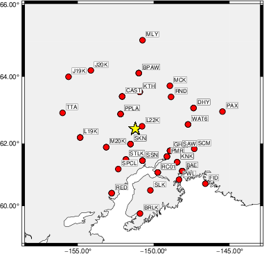
Waveform Inversion using wvfgrd96
The focal mechanism was determined using broadband seismic waveforms. The location of the event (star) and the
stations used for (red) the waveform inversion are shown in the next figure.
|
|
Location of broadband stations used for waveform inversion
|
The program wvfgrd96 was used with good traces observed at short distance to determine the focal mechanism, depth and seismic moment. This technique requires a high quality signal and well determined velocity model for the Green's functions. To the extent that these are the quality data, this type of mechanism should be preferred over the radiation pattern technique which requires the separate step of defining the pressure and tension quadrants and the correct strike.
The observed and predicted traces are filtered using the following gsac commands:
cut o DIST/3.5 -40 o DIST/3.5 +50
rtr
taper w 0.1
hp c 0.03 n 3
lp c 0.10 n 3
The results of this grid search are as follow:
           DEPTH  STK   DIP  RAKE   MW    FIT
WVFGRD96    2.0     0    50    10   3.67 0.1663
WVFGRD96    4.0   355    50     0   3.75 0.1927
WVFGRD96    6.0   355    60    -5   3.80 0.2152
WVFGRD96    8.0   355    55     0   3.88 0.2260
WVFGRD96   10.0   355    60     0   3.92 0.2308
WVFGRD96   12.0   355    60     5   3.95 0.2293
WVFGRD96   14.0    -5    60    10   3.98 0.2249
WVFGRD96   16.0     0    60    15   4.01 0.2175
WVFGRD96   18.0     0    65    25   4.03 0.2093
WVFGRD96   20.0     5    65    35   4.06 0.2067
WVFGRD96   22.0     5    65    35   4.09 0.2050
WVFGRD96   24.0   275    70   -20   4.12 0.2109
WVFGRD96   26.0   275    70   -20   4.14 0.2263
WVFGRD96   28.0   270    70   -20   4.17 0.2446
WVFGRD96   30.0   270    75   -25   4.19 0.2732
WVFGRD96   32.0   265    75   -25   4.22 0.3113
WVFGRD96   34.0   265    75   -30   4.24 0.3488
WVFGRD96   36.0   260    75   -30   4.26 0.3741
WVFGRD96   38.0   265    80   -30   4.29 0.3867
WVFGRD96   40.0   260    75   -40   4.37 0.4056
WVFGRD96   42.0   260    75   -40   4.39 0.4034
WVFGRD96   44.0   260    75   -40   4.41 0.4008
WVFGRD96   46.0   260    75   -40   4.42 0.4024
WVFGRD96   48.0   105    50    30   4.46 0.4080
WVFGRD96   50.0   105    50    30   4.47 0.4194
WVFGRD96   52.0   100    45    25   4.49 0.4296
WVFGRD96   54.0   230    80   -70   4.47 0.4393
WVFGRD96   56.0   230    80   -70   4.49 0.4564
WVFGRD96   58.0   230    85   -70   4.50 0.4746
WVFGRD96   60.0   225    85   -75   4.52 0.4945
WVFGRD96   62.0    50    90    70   4.53 0.5050
WVFGRD96   64.0    50    90    70   4.54 0.5235
WVFGRD96   66.0    45    90    75   4.56 0.5413
WVFGRD96   68.0    45    90    75   4.57 0.5582
WVFGRD96   70.0    45    90    75   4.58 0.5739
WVFGRD96   72.0   225    90   -75   4.59 0.5864
WVFGRD96   74.0    45    90    75   4.60 0.5992
WVFGRD96   76.0    45    90    75   4.61 0.6082
WVFGRD96   78.0    45    90    75   4.61 0.6175
WVFGRD96   80.0   225    90   -75   4.62 0.6234
WVFGRD96   82.0    45    90    75   4.63 0.6293
WVFGRD96   84.0   225    90   -75   4.63 0.6331
WVFGRD96   86.0    45    90    70   4.64 0.6360
WVFGRD96   88.0   225    90   -70   4.64 0.6411
WVFGRD96   90.0   225    90   -70   4.65 0.6436
WVFGRD96   92.0   225    90   -70   4.65 0.6464
WVFGRD96   94.0    45    90    70   4.66 0.6480
WVFGRD96   96.0    45    90    70   4.66 0.6486
WVFGRD96   98.0   225    90   -70   4.66 0.6480
WVFGRD96  100.0    45    90    70   4.67 0.6465
WVFGRD96  102.0    45    90    70   4.67 0.6432
WVFGRD96  104.0    45    90    70   4.67 0.6384
WVFGRD96  106.0   225    90   -70   4.67 0.6341
WVFGRD96  108.0   225    90   -70   4.67 0.6273
WVFGRD96  110.0   225    90   -70   4.67 0.6213
WVFGRD96  112.0   225    90   -70   4.67 0.6139
WVFGRD96  114.0    45    90    70   4.67 0.6055
WVFGRD96  116.0    45    90    70   4.67 0.5965
WVFGRD96  118.0    45    90    70   4.67 0.5874
WVFGRD96  120.0    50    85    70   4.66 0.5765
WVFGRD96  122.0    50    85    70   4.66 0.5682
WVFGRD96  124.0    50    85    70   4.66 0.5597
WVFGRD96  126.0    50    85    70   4.66 0.5496
WVFGRD96  128.0    50    85    70   4.66 0.5393
WVFGRD96  130.0    50    85    65   4.66 0.5301
WVFGRD96  132.0   225    90   -70   4.66 0.5120
WVFGRD96  134.0    50    85    65   4.66 0.5114
WVFGRD96  136.0    50    85    65   4.66 0.5023
WVFGRD96  138.0    50    85    65   4.65 0.4885
WVFGRD96  140.0    50    85    65   4.64 0.4447
WVFGRD96  142.0    55    80    60   4.61 0.3882
WVFGRD96  144.0    50    80    60   4.59 0.3343
WVFGRD96  146.0    55    75    55   4.56 0.2856
WVFGRD96  148.0    85    45    40   4.53 0.2543
The best solution is
WVFGRD96 96.0 45 90 70 4.66 0.6486
The mechanism corresponding to the best fit is
|
|
Figure 1. Waveform inversion focal mechanism
|
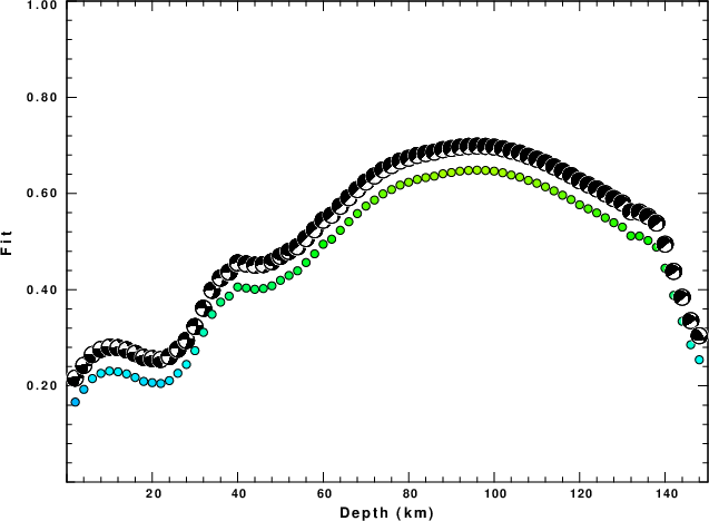
The best fit as a function of depth is given in the following figure:
|
|
Figure 2. Depth sensitivity for waveform mechanism
|
The comparison of the observed and predicted waveforms is given in the next figure. The red traces are the observed and the blue are the predicted.
Each observed-predicted component is plotted to the same scale and peak amplitudes are indicated by the numbers to the left of each trace. A pair of numbers is given in black at the right of each predicted traces. The upper number it the time shift required for maximum correlation between the observed and predicted traces. This time shift is required because the synthetics are not computed at exactly the same distance as the observed, the velocity model used in the predictions may not be perfect and the epicentral parameters may be be off.
A positive time shift indicates that the prediction is too fast and should be delayed to match the observed trace (shift to the right in this figure). A negative value indicates that the prediction is too slow. The lower number gives the percentage of variance reduction to characterize the individual goodness of fit (100% indicates a perfect fit).
The bandpass filter used in the processing and for the display was
cut o DIST/3.5 -40 o DIST/3.5 +50
rtr
taper w 0.1
hp c 0.03 n 3
lp c 0.10 n 3
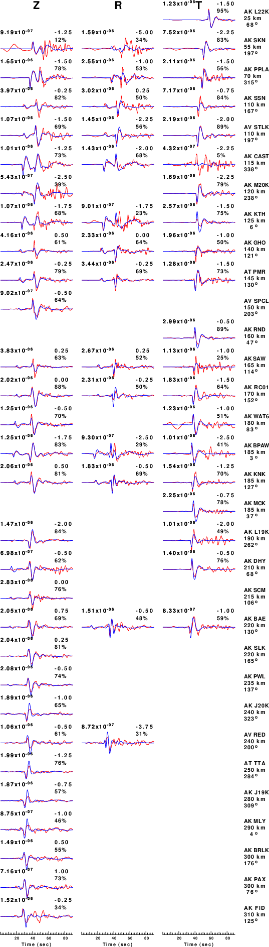
|
|
Figure 3. Waveform comparison for selected depth. Red: observed; Blue - predicted. The time shift with respect to the model prediction is indicated. The percent of fit is also indicated. The time scale is relative to the first trace sample.
|
|
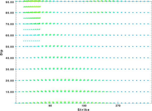
|
Focal mechanism sensitivity at the preferred depth. The red color indicates a very good fit to the waveforms.
Each solution is plotted as a vector at a given value of strike and dip with the angle of the vector representing the rake angle, measured, with respect to the upward vertical (N) in the figure.
|
A check on the assumed source location is possible by looking at the time shifts between the observed and predicted traces. The time shifts for waveform matching arise for several reasons:
- The origin time and epicentral distance are incorrect
- The velocity model used for the inversion is incorrect
- The velocity model used to define the P-arrival time is not the
same as the velocity model used for the waveform inversion
(assuming that the initial trace alignment is based on the
P arrival time)
Assuming only a mislocation, the time shifts are fit to a functional form:
Time_shift = A + B cos Azimuth + C Sin Azimuth
The time shifts for this inversion lead to the next figure:
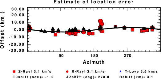
The derived shift in origin time and epicentral coordinates are given at the bottom of the figure.
Velocity Model
The WUS.model used for the waveform synthetic seismograms and for the surface wave eigenfunctions and dispersion is as follows
(The format is in the model96 format of Computer Programs in Seismology).
MODEL.01
Model after     8 iterations
ISOTROPIC
KGS
FLAT EARTH
1-D
CONSTANT VELOCITY
LINE08
LINE09
LINE10
LINE11
      H(KM)   VP(KM/S)   VS(KM/S) RHO(GM/CC)         QP         QS       ETAP       ETAS      FREFP      FREFS
     1.9000     3.4065     2.0089     2.2150  0.302E-02  0.679E-02   0.00       0.00       1.00       1.00
     6.1000     5.5445     3.2953     2.6089  0.349E-02  0.784E-02   0.00       0.00       1.00       1.00
    13.0000     6.2708     3.7396     2.7812  0.212E-02  0.476E-02   0.00       0.00       1.00       1.00
    19.0000     6.4075     3.7680     2.8223  0.111E-02  0.249E-02   0.00       0.00       1.00       1.00
     0.0000     7.9000     4.6200     3.2760  0.164E-10  0.370E-10   0.00       0.00       1.00       1.00
Last Changed Thu Aug 14 06:59:37 EDT 2025