Location
Location ANSS
The ANSS event ID is us6000qhk7 and the event page is at
https://earthquake.usgs.gov/earthquakes/eventpage/us6000qhk7/executive.
2025/06/03 04:38:59 44.339 -114.988 13.8 3.8 Idaho
Focal Mechanism
 USGS/SLU Moment Tensor Solution
 ENS  2025/06/03 04:38:59.0  44.34 -114.99  13.8 3.8 Idaho

 Stations used:
   IE.BCYI IE.NPRI IW.DLMT IW.IMW IW.LOHW IW.MFID IW.MOOW
   IW.PLID MB.BCMT MB.BDMT MB.BNMT MB.CPMT MB.ECMT MB.FCMT
   MB.GBMT MB.HRY MB.LIMT MB.LRM MB.ODMT MB.SMMT MB.SRMT
   MB.SXMT MB.WCMT UO.JAZZ UO.PRONG US.BMO US.BOZ US.HLID
   US.HWUT US.WVOR UU.BEID UU.BGU UU.HVU UU.SPU UW.BRAN
   UW.BURN UW.IRON UW.IZEE UW.LBRT UW.LMONT UW.LNO UW.PHIN
   UW.TUCA UW.WOLL WW.BILL WW.CNCL WW.CTNW WW.IRMR WW.TYLR
   WY.YDD WY.YFT WY.YHB WY.YMR

 Filtering commands used:
   cut o DIST/3.3 -40 o DIST/3.3 +50
   rtr
   taper w 0.1
   hp c 0.03 n 3
   lp c 0.10 n 3
   br c 0.12 0.25 n 4 p 2

 Best Fitting Double Couple
  Mo = 4.32e+21 dyne-cm
  Mw = 3.69
  Z  = 10 km
  Plane   Strike  Dip  Rake
   NP1      150    80   -55
   NP2      254    36   -163
  Principal Axes:
   Axis    Value   Plunge  Azimuth
    T   4.32e+21     27     213
    N   0.00e+00     34     323
    P  -4.32e+21     44      94

 Moment Tensor: (dyne-cm)
    Component   Value
       Mxx     2.41e+21
       Mxy     1.74e+21
       Mxz    -1.29e+21
       Myy    -1.20e+21
       Myz    -3.09e+21
       Mzz    -1.21e+21


                     ##############
                 -#####################
              ----########################
             ------########################
           --------###------------------#####
          --------##-----------------------###
         -------#####-------------------------#
        ------########-------------------------#
        ----###########-------------------------
       ----#############-------------------------
       ---###############-------------   --------
       --#################------------ P --------
       --##################-----------   --------
        ####################--------------------
        #####################-------------------
         #####################-----------------
          ######################--------------
           #######   ############------------
             ##### T #############---------
              ####   ###############------
                 #####################-
                     ##############


 Global CMT Convention Moment Tensor:
      R          T          P
 -1.21e+21  -1.29e+21   3.09e+21
 -1.29e+21   2.41e+21  -1.74e+21
  3.09e+21  -1.74e+21  -1.20e+21


Details of the solution is found at

http://www.eas.slu.edu/eqc/eqc_mt/MECH.NA/20250603043859/index.html
|
Preferred Solution
The preferred solution from an analysis of the surface-wave spectral amplitude radiation pattern, waveform inversion or first motion observations is
      STK = 150
      DIP = 80
     RAKE = -55
       MW = 3.69
       HS = 10.0
The NDK file is 20250603043859.ndk
The waveform inversion is preferred.
Moment Tensor Comparison
The following compares this source inversion to those provided by others. The purpose is to look for major differences and also to note slight differences that might be inherent to the processing procedure. For completeness the USGS/SLU solution is repeated from above.
| SLU |
USGSMWR |
 USGS/SLU Moment Tensor Solution
 ENS  2025/06/03 04:38:59.0  44.34 -114.99  13.8 3.8 Idaho

 Stations used:
   IE.BCYI IE.NPRI IW.DLMT IW.IMW IW.LOHW IW.MFID IW.MOOW
   IW.PLID MB.BCMT MB.BDMT MB.BNMT MB.CPMT MB.ECMT MB.FCMT
   MB.GBMT MB.HRY MB.LIMT MB.LRM MB.ODMT MB.SMMT MB.SRMT
   MB.SXMT MB.WCMT UO.JAZZ UO.PRONG US.BMO US.BOZ US.HLID
   US.HWUT US.WVOR UU.BEID UU.BGU UU.HVU UU.SPU UW.BRAN
   UW.BURN UW.IRON UW.IZEE UW.LBRT UW.LMONT UW.LNO UW.PHIN
   UW.TUCA UW.WOLL WW.BILL WW.CNCL WW.CTNW WW.IRMR WW.TYLR
   WY.YDD WY.YFT WY.YHB WY.YMR

 Filtering commands used:
   cut o DIST/3.3 -40 o DIST/3.3 +50
   rtr
   taper w 0.1
   hp c 0.03 n 3
   lp c 0.10 n 3
   br c 0.12 0.25 n 4 p 2

 Best Fitting Double Couple
  Mo = 4.32e+21 dyne-cm
  Mw = 3.69
  Z  = 10 km
  Plane   Strike  Dip  Rake
   NP1      150    80   -55
   NP2      254    36   -163
  Principal Axes:
   Axis    Value   Plunge  Azimuth
    T   4.32e+21     27     213
    N   0.00e+00     34     323
    P  -4.32e+21     44      94

 Moment Tensor: (dyne-cm)
    Component   Value
       Mxx     2.41e+21
       Mxy     1.74e+21
       Mxz    -1.29e+21
       Myy    -1.20e+21
       Myz    -3.09e+21
       Mzz    -1.21e+21


                     ##############
                 -#####################
              ----########################
             ------########################
           --------###------------------#####
          --------##-----------------------###
         -------#####-------------------------#
        ------########-------------------------#
        ----###########-------------------------
       ----#############-------------------------
       ---###############-------------   --------
       --#################------------ P --------
       --##################-----------   --------
        ####################--------------------
        #####################-------------------
         #####################-----------------
          ######################--------------
           #######   ############------------
             ##### T #############---------
              ####   ###############------
                 #####################-
                     ##############


 Global CMT Convention Moment Tensor:
      R          T          P
 -1.21e+21  -1.29e+21   3.09e+21
 -1.29e+21   2.41e+21  -1.74e+21
  3.09e+21  -1.74e+21  -1.20e+21


Details of the solution is found at

http://www.eas.slu.edu/eqc/eqc_mt/MECH.NA/20250603043859/index.html
|
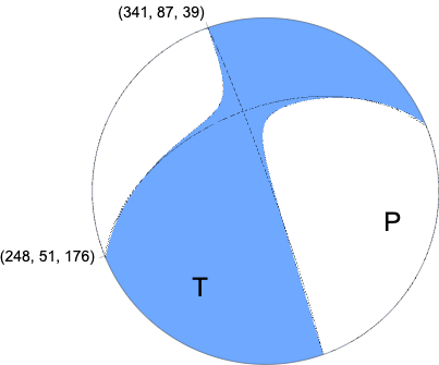
Regional Moment Tensor (Mwr)
Moment 4.567e+14 N-m
Magnitude 3.71 Mwr
Depth 15.0 km
Percent DC 92%
Half Duration -
Catalog US
Data Source US
Contributor US
Nodal Planes
Plane	Strike	Dip	Rake
NP1	248	51	176
NP2	341	87	39
Principal Axes
Axis	Value	Plunge	Azimuth
T	4.470e+14	29	212
N	0.189e+14	50	344
P	-4.659e+14	24	107
|
Magnitudes
Given the availability of digital waveforms for determination of the moment tensor, this section documents the added processing leading to mLg, if appropriate to the region, and ML by application of the respective IASPEI formulae. As a research study, the linear distance term of the IASPEI formula
for ML is adjusted to remove a linear distance trend in residuals to give a regionally defined ML. The defined ML uses horizontal component recordings, but the same procedure is applied to the vertical components since there may be some interest in vertical component ground motions. Residual plots versus distance may indicate interesting features of ground motion scaling in some distance ranges. A residual plot of the regionalized magnitude is given as a function of distance and azimuth, since data sets may transcend different wave propagation provinces.
ML Magnitude
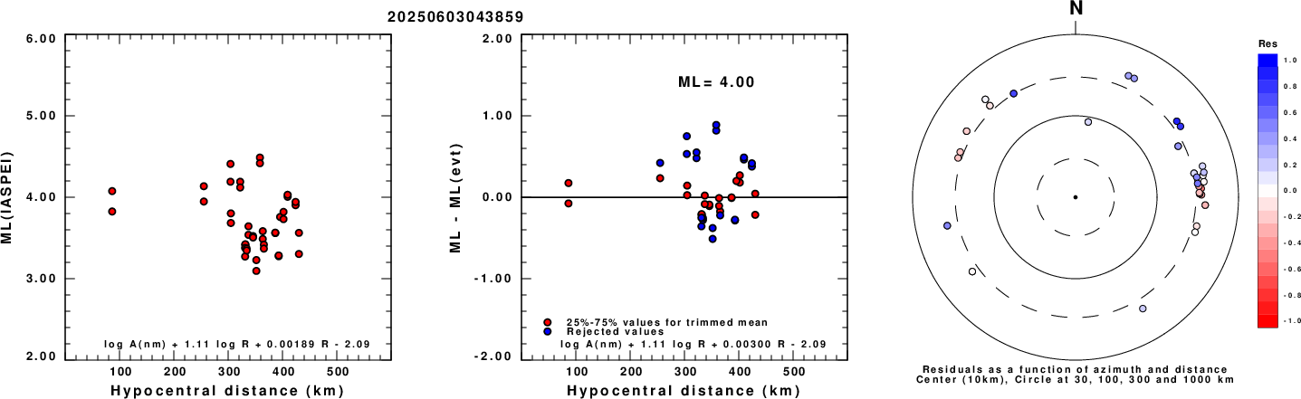
Left: ML computed using the IASPEI formula for Horizontal components. Center: ML residuals computed using a modified IASPEI formula that accounts for path specific attenuation; the values used for the trimmed mean are indicated. The ML relation used for each figure is given at the bottom of each plot.
Right: Residuals from new relation as a function of distance and azimuth.
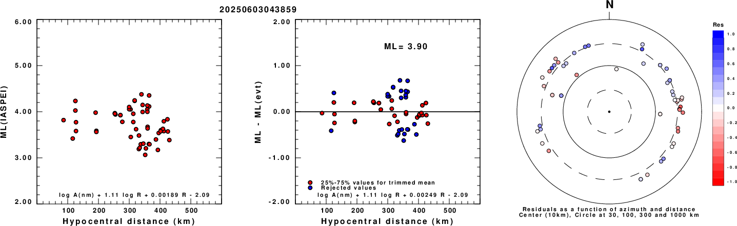
Left: ML computed using the IASPEI formula for Vertical components (research). Center: ML residuals computed using a modified IASPEI formula that accounts for path specific attenuation; the values used for the trimmed mean are indicated. The ML relation used for each figure is given at the bottom of each plot.
Right: Residuals from new relation as a function of distance and azimuth.
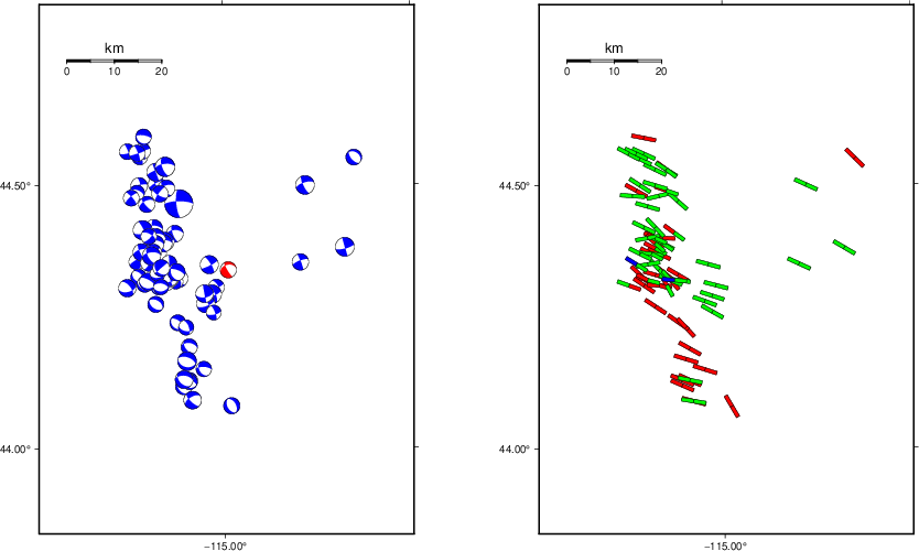
Context
The left panel of the next figure presents the focal mechanism for this earthquake (red) in the context of other nearby events (blue) in the SLU Moment Tensor Catalog. The right panel shows the inferred direction of maximum compressive stress and the type of faulting (green is strike-slip, red is normal, blue is thrust; oblique is shown by a combination of colors). Thus context plot is useful for assessing the appropriateness of the moment tensor of this event.
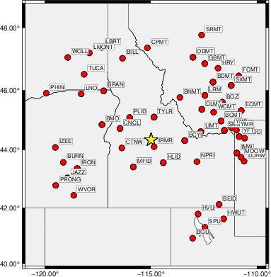
Waveform Inversion using wvfgrd96
The focal mechanism was determined using broadband seismic waveforms. The location of the event (star) and the
stations used for (red) the waveform inversion are shown in the next figure.
|
|
Location of broadband stations used for waveform inversion
|
The program wvfgrd96 was used with good traces observed at short distance to determine the focal mechanism, depth and seismic moment. This technique requires a high quality signal and well determined velocity model for the Green's functions. To the extent that these are the quality data, this type of mechanism should be preferred over the radiation pattern technique which requires the separate step of defining the pressure and tension quadrants and the correct strike.
The observed and predicted traces are filtered using the following gsac commands:
cut o DIST/3.3 -40 o DIST/3.3 +50
rtr
taper w 0.1
hp c 0.03 n 3
lp c 0.10 n 3
br c 0.12 0.25 n 4 p 2
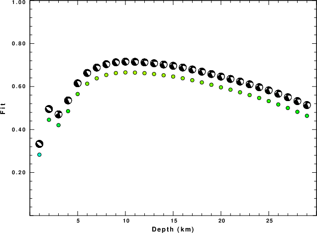
The results of this grid search are as follow:
           DEPTH  STK   DIP  RAKE   MW    FIT
WVFGRD96    1.0   130    45   -90   3.34 0.2832
WVFGRD96    2.0   310    45   -85   3.52 0.4455
WVFGRD96    3.0   335    70    25   3.46 0.4206
WVFGRD96    4.0   155    85   -60   3.60 0.4855
WVFGRD96    5.0   155    85   -60   3.62 0.5652
WVFGRD96    6.0   150    80   -60   3.63 0.6132
WVFGRD96    7.0   150    80   -55   3.63 0.6382
WVFGRD96    8.0   150    80   -60   3.69 0.6540
WVFGRD96    9.0   145    75   -60   3.69 0.6627
WVFGRD96   10.0   150    80   -55   3.69 0.6657
WVFGRD96   11.0   150    80   -55   3.69 0.6648
WVFGRD96   12.0   150    80   -50   3.69 0.6623
WVFGRD96   13.0   150    80   -50   3.70 0.6582
WVFGRD96   14.0   155    85   -45   3.71 0.6524
WVFGRD96   15.0   155    85   -45   3.72 0.6464
WVFGRD96   16.0   155    85   -45   3.73 0.6385
WVFGRD96   17.0   155    85   -45   3.73 0.6294
WVFGRD96   18.0   155    85   -45   3.74 0.6192
WVFGRD96   19.0   155    85   -45   3.75 0.6082
WVFGRD96   20.0   335    90    45   3.76 0.5963
WVFGRD96   21.0   155    90   -45   3.77 0.5854
WVFGRD96   22.0   155    90   -45   3.78 0.5733
WVFGRD96   23.0   335    90    45   3.79 0.5605
WVFGRD96   24.0   335    90    45   3.80 0.5469
WVFGRD96   25.0   335    90    45   3.81 0.5324
WVFGRD96   26.0   335    90    45   3.82 0.5167
WVFGRD96   27.0   335    90    45   3.82 0.5003
WVFGRD96   28.0   335    90    45   3.83 0.4824
WVFGRD96   29.0   335    85    45   3.83 0.4639
The best solution is
WVFGRD96 10.0 150 80 -55 3.69 0.6657
The mechanism corresponding to the best fit is
|
|
Figure 1. Waveform inversion focal mechanism
|
The best fit as a function of depth is given in the following figure:
|
|
Figure 2. Depth sensitivity for waveform mechanism
|
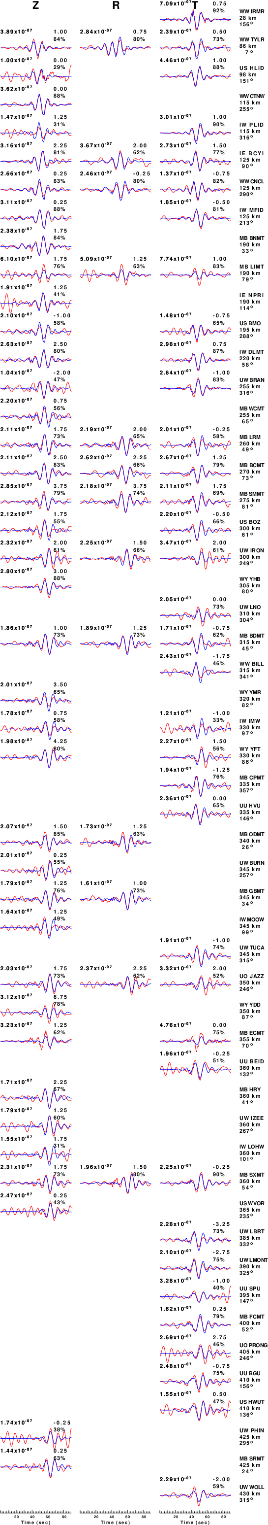
The comparison of the observed and predicted waveforms is given in the next figure. The red traces are the observed and the blue are the predicted.
Each observed-predicted component is plotted to the same scale and peak amplitudes are indicated by the numbers to the left of each trace. A pair of numbers is given in black at the right of each predicted traces. The upper number it the time shift required for maximum correlation between the observed and predicted traces. This time shift is required because the synthetics are not computed at exactly the same distance as the observed, the velocity model used in the predictions may not be perfect and the epicentral parameters may be be off.
A positive time shift indicates that the prediction is too fast and should be delayed to match the observed trace (shift to the right in this figure). A negative value indicates that the prediction is too slow. The lower number gives the percentage of variance reduction to characterize the individual goodness of fit (100% indicates a perfect fit).
The bandpass filter used in the processing and for the display was
cut o DIST/3.3 -40 o DIST/3.3 +50
rtr
taper w 0.1
hp c 0.03 n 3
lp c 0.10 n 3
br c 0.12 0.25 n 4 p 2
|
|
Figure 3. Waveform comparison for selected depth. Red: observed; Blue - predicted. The time shift with respect to the model prediction is indicated. The percent of fit is also indicated. The time scale is relative to the first trace sample.
|
|
|
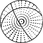
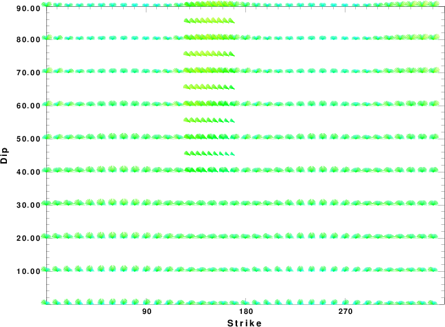
Focal mechanism sensitivity at the preferred depth. The red color indicates a very good fit to the waveforms.
Each solution is plotted as a vector at a given value of strike and dip with the angle of the vector representing the rake angle, measured, with respect to the upward vertical (N) in the figure.
|
A check on the assumed source location is possible by looking at the time shifts between the observed and predicted traces. The time shifts for waveform matching arise for several reasons:
- The origin time and epicentral distance are incorrect
- The velocity model used for the inversion is incorrect
- The velocity model used to define the P-arrival time is not the
same as the velocity model used for the waveform inversion
(assuming that the initial trace alignment is based on the
P arrival time)
Assuming only a mislocation, the time shifts are fit to a functional form:
Time_shift = A + B cos Azimuth + C Sin Azimuth
The time shifts for this inversion lead to the next figure:
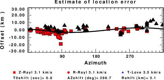
The derived shift in origin time and epicentral coordinates are given at the bottom of the figure.
Velocity Model
The WUS.model used for the waveform synthetic seismograms and for the surface wave eigenfunctions and dispersion is as follows
(The format is in the model96 format of Computer Programs in Seismology).
MODEL.01
Model after     8 iterations
ISOTROPIC
KGS
FLAT EARTH
1-D
CONSTANT VELOCITY
LINE08
LINE09
LINE10
LINE11
      H(KM)   VP(KM/S)   VS(KM/S) RHO(GM/CC)         QP         QS       ETAP       ETAS      FREFP      FREFS
     1.9000     3.4065     2.0089     2.2150  0.302E-02  0.679E-02   0.00       0.00       1.00       1.00
     6.1000     5.5445     3.2953     2.6089  0.349E-02  0.784E-02   0.00       0.00       1.00       1.00
    13.0000     6.2708     3.7396     2.7812  0.212E-02  0.476E-02   0.00       0.00       1.00       1.00
    19.0000     6.4075     3.7680     2.8223  0.111E-02  0.249E-02   0.00       0.00       1.00       1.00
     0.0000     7.9000     4.6200     3.2760  0.164E-10  0.370E-10   0.00       0.00       1.00       1.00
Last Changed Tue Jun 3 06:41:20 CDT 2025