Location
Location ANSS
The ANSS event ID is ak0255iimhly and the event page is at
https://earthquake.usgs.gov/earthquakes/eventpage/ak0255iimhly/executive.
2025/04/30 03:58:52 59.715 -152.729 87.2 4.0 Alaska
Focal Mechanism
 USGS/SLU Moment Tensor Solution
 ENS  2025/04/30 03:58:52:0  59.72 -152.73  87.2 4.0 Alaska

 Stations used:
   AK.CAPN AK.GHO AK.N18K AK.O18K AK.O19K AK.P17K AK.PWL
   AK.RC01 AK.SLK AK.SSN AK.SWD AT.PMR AV.ACH AV.RED AV.SPCL
   AV.STLK II.KDAK

 Filtering commands used:
   cut o DIST/3.5 -40 o DIST/3.5 +50
   rtr
   taper w 0.1
   hp c 0.03 n 3
   lp c 0.08 n 3

 Best Fitting Double Couple
  Mo = 2.60e+22 dyne-cm
  Mw = 4.21
  Z  = 120 km
  Plane   Strike  Dip  Rake
   NP1      310    73   148
   NP2       50    60    20
  Principal Axes:
   Axis    Value   Plunge  Azimuth
    T   2.60e+22     34     266
    N   0.00e+00     54     104
    P  -2.60e+22      8       2

 Moment Tensor: (dyne-cm)
    Component   Value
       Mxx    -2.54e+22
       Mxy     1.18e+20
       Mxz    -4.45e+21
       Myy     1.77e+22
       Myz    -1.22e+22
       Mzz     7.70e+21


                     ------ P -----
                 ----------   ---------
              ----------------------------
             ------------------------------
           ######---------------------------#
          ###########-----------------------##
         ###############-------------------####
        ###################---------------######
        #####################------------#######
       #########################--------#########
       ######   ##################-----##########
       ###### T ####################--###########
       ######   ####################-############
        ##########################-----#########
        ########################--------########
         #####################------------#####
          #################----------------###
           ###########----------------------#
             ------------------------------
              ----------------------------
                 ----------------------
                     --------------


 Global CMT Convention Moment Tensor:
      R          T          P
  7.70e+21  -4.45e+21   1.22e+22
 -4.45e+21  -2.54e+22  -1.18e+20
  1.22e+22  -1.18e+20   1.77e+22


Details of the solution is found at

http://www.eas.slu.edu/eqc/eqc_mt/MECH.NA/20250430035852/index.html
|
Preferred Solution
The preferred solution from an analysis of the surface-wave spectral amplitude radiation pattern, waveform inversion or first motion observations is
      STK = 50
      DIP = 60
     RAKE = 20
       MW = 4.21
       HS = 120.0
The NDK file is 20250430035852.ndk
The waveform inversion is preferred.
Magnitudes
Given the availability of digital waveforms for determination of the moment tensor, this section documents the added processing leading to mLg, if appropriate to the region, and ML by application of the respective IASPEI formulae. As a research study, the linear distance term of the IASPEI formula
for ML is adjusted to remove a linear distance trend in residuals to give a regionally defined ML. The defined ML uses horizontal component recordings, but the same procedure is applied to the vertical components since there may be some interest in vertical component ground motions. Residual plots versus distance may indicate interesting features of ground motion scaling in some distance ranges. A residual plot of the regionalized magnitude is given as a function of distance and azimuth, since data sets may transcend different wave propagation provinces.
ML Magnitude
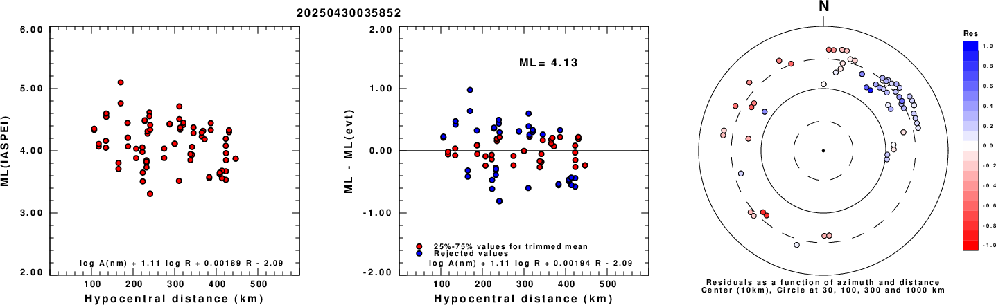
Left: ML computed using the IASPEI formula for Horizontal components. Center: ML residuals computed using a modified IASPEI formula that accounts for path specific attenuation; the values used for the trimmed mean are indicated. The ML relation used for each figure is given at the bottom of each plot.
Right: Residuals from new relation as a function of distance and azimuth.
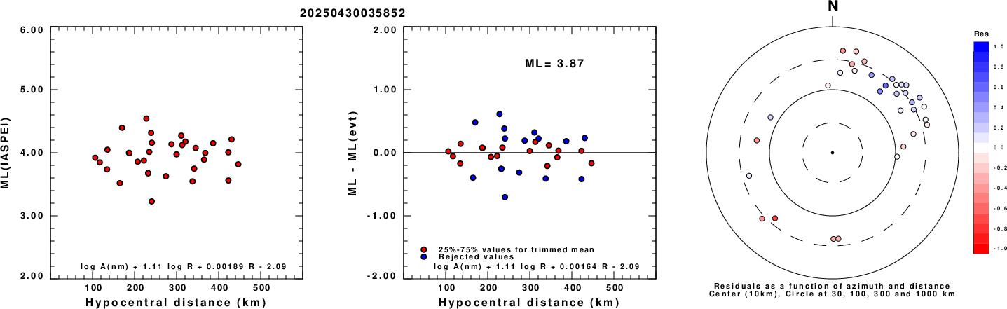
Left: ML computed using the IASPEI formula for Vertical components (research). Center: ML residuals computed using a modified IASPEI formula that accounts for path specific attenuation; the values used for the trimmed mean are indicated. The ML relation used for each figure is given at the bottom of each plot.
Right: Residuals from new relation as a function of distance and azimuth.
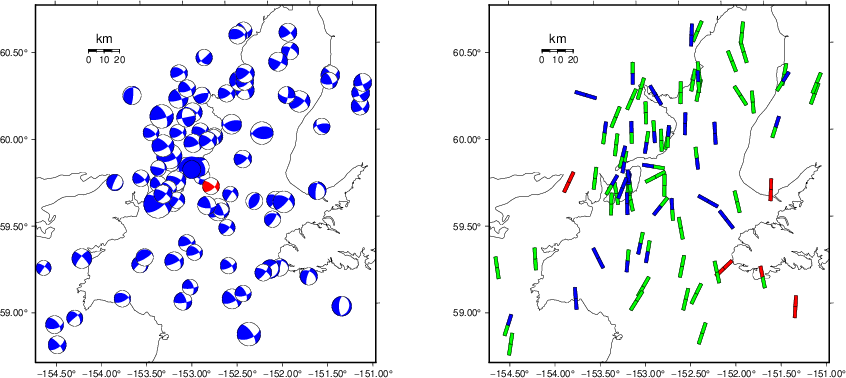
Context
The left panel of the next figure presents the focal mechanism for this earthquake (red) in the context of other nearby events (blue) in the SLU Moment Tensor Catalog. The right panel shows the inferred direction of maximum compressive stress and the type of faulting (green is strike-slip, red is normal, blue is thrust; oblique is shown by a combination of colors). Thus context plot is useful for assessing the appropriateness of the moment tensor of this event.
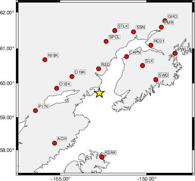
Waveform Inversion using wvfgrd96
The focal mechanism was determined using broadband seismic waveforms. The location of the event (star) and the
stations used for (red) the waveform inversion are shown in the next figure.
|
|
Location of broadband stations used for waveform inversion
|
The program wvfgrd96 was used with good traces observed at short distance to determine the focal mechanism, depth and seismic moment. This technique requires a high quality signal and well determined velocity model for the Green's functions. To the extent that these are the quality data, this type of mechanism should be preferred over the radiation pattern technique which requires the separate step of defining the pressure and tension quadrants and the correct strike.
The observed and predicted traces are filtered using the following gsac commands:
cut o DIST/3.5 -40 o DIST/3.5 +50
rtr
taper w 0.1
hp c 0.03 n 3
lp c 0.08 n 3
The results of this grid search are as follow:
           DEPTH  STK   DIP  RAKE   MW    FIT
WVFGRD96    2.0   305    65   -25   3.22 0.0796
WVFGRD96    4.0   310    75    10   3.26 0.0875
WVFGRD96    6.0   310    65    15   3.34 0.0934
WVFGRD96    8.0   315    60    20   3.41 0.0967
WVFGRD96   10.0    35    80   -50   3.49 0.0992
WVFGRD96   12.0    40    85   -50   3.52 0.1021
WVFGRD96   14.0   225    90    50   3.55 0.1042
WVFGRD96   16.0   225    90    45   3.57 0.1072
WVFGRD96   18.0    45    90   -45   3.60 0.1115
WVFGRD96   20.0    45    90   -45   3.63 0.1164
WVFGRD96   22.0    40    90   -45   3.66 0.1219
WVFGRD96   24.0    40    90   -45   3.69 0.1272
WVFGRD96   26.0   225    85    40   3.71 0.1326
WVFGRD96   28.0    40    85   -45   3.74 0.1381
WVFGRD96   30.0    40    85   -45   3.76 0.1427
WVFGRD96   32.0   225    90    40   3.77 0.1456
WVFGRD96   34.0    45    90   -40   3.79 0.1480
WVFGRD96   36.0   225    90    40   3.81 0.1497
WVFGRD96   38.0    45    90   -35   3.84 0.1521
WVFGRD96   40.0    45    85   -50   3.95 0.1567
WVFGRD96   42.0    45    85   -45   3.96 0.1584
WVFGRD96   44.0    45    85   -45   3.98 0.1595
WVFGRD96   46.0    45    80   -40   3.99 0.1602
WVFGRD96   48.0    45    80   -40   4.01 0.1606
WVFGRD96   50.0    45    75   -35   4.03 0.1615
WVFGRD96   52.0    45    75   -35   4.04 0.1637
WVFGRD96   54.0    50    75   -30   4.06 0.1663
WVFGRD96   56.0    50    75   -25   4.07 0.1695
WVFGRD96   58.0    50    70   -25   4.09 0.1733
WVFGRD96   60.0    50    60   -10   4.09 0.1795
WVFGRD96   62.0    50    60    -5   4.10 0.1861
WVFGRD96   64.0    50    60    -5   4.11 0.1925
WVFGRD96   66.0    50    60    -5   4.12 0.1981
WVFGRD96   68.0    50    60    -5   4.13 0.2037
WVFGRD96   70.0    50    55    -5   4.15 0.2098
WVFGRD96   72.0    50    55    -5   4.16 0.2146
WVFGRD96   74.0    50    55    -5   4.16 0.2195
WVFGRD96   76.0    50    55     0   4.16 0.2240
WVFGRD96   78.0    50    55     0   4.17 0.2284
WVFGRD96   80.0    50    55     0   4.18 0.2320
WVFGRD96   82.0    50    55     0   4.18 0.2359
WVFGRD96   84.0    50    55     5   4.18 0.2385
WVFGRD96   86.0    50    55     5   4.18 0.2421
WVFGRD96   88.0    50    55     5   4.19 0.2450
WVFGRD96   90.0    50    55     5   4.19 0.2467
WVFGRD96   92.0    50    55    10   4.19 0.2494
WVFGRD96   94.0    50    55    10   4.20 0.2517
WVFGRD96   96.0    50    55    10   4.20 0.2534
WVFGRD96   98.0    50    55    10   4.20 0.2547
WVFGRD96  100.0    50    55    10   4.21 0.2561
WVFGRD96  102.0    50    55    15   4.21 0.2575
WVFGRD96  104.0    50    55    15   4.21 0.2589
WVFGRD96  106.0    50    55    15   4.21 0.2599
WVFGRD96  108.0    50    55    15   4.22 0.2604
WVFGRD96  110.0    50    60    20   4.20 0.2608
WVFGRD96  112.0    50    60    20   4.20 0.2613
WVFGRD96  114.0    50    60    20   4.20 0.2616
WVFGRD96  116.0    50    60    20   4.21 0.2617
WVFGRD96  118.0    50    60    20   4.21 0.2617
WVFGRD96  120.0    50    60    20   4.21 0.2618
WVFGRD96  122.0    50    60    25   4.21 0.2616
WVFGRD96  124.0    50    60    25   4.21 0.2613
WVFGRD96  126.0    50    60    25   4.21 0.2611
WVFGRD96  128.0    50    60    25   4.22 0.2608
WVFGRD96  130.0   210    90   -75   4.27 0.2612
WVFGRD96  132.0    30    90    75   4.27 0.2612
WVFGRD96  134.0   210    90   -75   4.27 0.2611
WVFGRD96  136.0    30    90    75   4.27 0.2606
WVFGRD96  138.0    30    90    75   4.27 0.2601
WVFGRD96  140.0   210    90   -75   4.26 0.2594
WVFGRD96  142.0    30    90    75   4.26 0.2584
WVFGRD96  144.0   210    90   -75   4.26 0.2569
WVFGRD96  146.0    35    85    75   4.26 0.2557
WVFGRD96  148.0   210    90   -70   4.24 0.2541
The best solution is
WVFGRD96 120.0 50 60 20 4.21 0.2618
The mechanism corresponding to the best fit is
|
|
Figure 1. Waveform inversion focal mechanism
|
The best fit as a function of depth is given in the following figure:
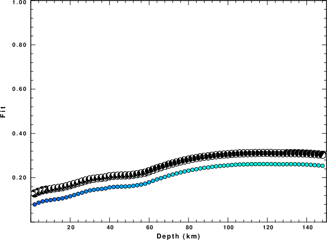
|
|
Figure 2. Depth sensitivity for waveform mechanism
|
The comparison of the observed and predicted waveforms is given in the next figure. The red traces are the observed and the blue are the predicted.
Each observed-predicted component is plotted to the same scale and peak amplitudes are indicated by the numbers to the left of each trace. A pair of numbers is given in black at the right of each predicted traces. The upper number it the time shift required for maximum correlation between the observed and predicted traces. This time shift is required because the synthetics are not computed at exactly the same distance as the observed, the velocity model used in the predictions may not be perfect and the epicentral parameters may be be off.
A positive time shift indicates that the prediction is too fast and should be delayed to match the observed trace (shift to the right in this figure). A negative value indicates that the prediction is too slow. The lower number gives the percentage of variance reduction to characterize the individual goodness of fit (100% indicates a perfect fit).
The bandpass filter used in the processing and for the display was
cut o DIST/3.5 -40 o DIST/3.5 +50
rtr
taper w 0.1
hp c 0.03 n 3
lp c 0.08 n 3
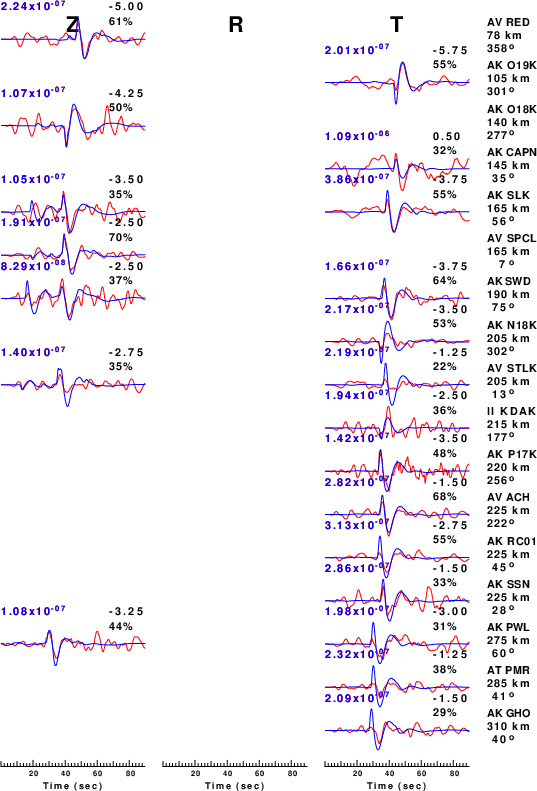
|
|
Figure 3. Waveform comparison for selected depth. Red: observed; Blue - predicted. The time shift with respect to the model prediction is indicated. The percent of fit is also indicated. The time scale is relative to the first trace sample.
|
|
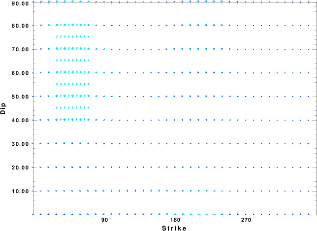
|
Focal mechanism sensitivity at the preferred depth. The red color indicates a very good fit to the waveforms.
Each solution is plotted as a vector at a given value of strike and dip with the angle of the vector representing the rake angle, measured, with respect to the upward vertical (N) in the figure.
|
A check on the assumed source location is possible by looking at the time shifts between the observed and predicted traces. The time shifts for waveform matching arise for several reasons:
- The origin time and epicentral distance are incorrect
- The velocity model used for the inversion is incorrect
- The velocity model used to define the P-arrival time is not the
same as the velocity model used for the waveform inversion
(assuming that the initial trace alignment is based on the
P arrival time)
Assuming only a mislocation, the time shifts are fit to a functional form:
Time_shift = A + B cos Azimuth + C Sin Azimuth
The time shifts for this inversion lead to the next figure:
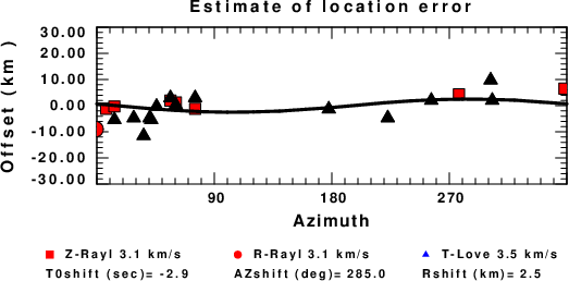
The derived shift in origin time and epicentral coordinates are given at the bottom of the figure.
Velocity Model
The WUS.model used for the waveform synthetic seismograms and for the surface wave eigenfunctions and dispersion is as follows
(The format is in the model96 format of Computer Programs in Seismology).
MODEL.01
Model after     8 iterations
ISOTROPIC
KGS
FLAT EARTH
1-D
CONSTANT VELOCITY
LINE08
LINE09
LINE10
LINE11
      H(KM)   VP(KM/S)   VS(KM/S) RHO(GM/CC)         QP         QS       ETAP       ETAS      FREFP      FREFS
     1.9000     3.4065     2.0089     2.2150  0.302E-02  0.679E-02   0.00       0.00       1.00       1.00
     6.1000     5.5445     3.2953     2.6089  0.349E-02  0.784E-02   0.00       0.00       1.00       1.00
    13.0000     6.2708     3.7396     2.7812  0.212E-02  0.476E-02   0.00       0.00       1.00       1.00
    19.0000     6.4075     3.7680     2.8223  0.111E-02  0.249E-02   0.00       0.00       1.00       1.00
     0.0000     7.9000     4.6200     3.2760  0.164E-10  0.370E-10   0.00       0.00       1.00       1.00
Last Changed Wed Apr 30 09:14:09 CDT 2025