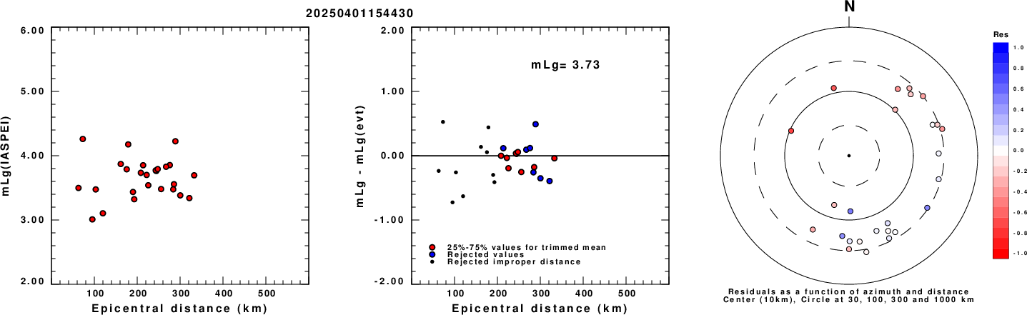
Left: mLg computed using the IASPEI formula. Center: mLg residuals versus epicentral distance ; the values used for the trimmed mean magnitude estimate are indicated. Right: residuals as a function of distance and azimuth.
The ANSS event ID is ak02546r3kto and the event page is at https://earthquake.usgs.gov/earthquakes/eventpage/ak02546r3kto/executive.
2025/04/01 15:44:30 63.060 -150.361 106.2 3.7 Alaska
 USGS/SLU Moment Tensor Solution
 ENS  2025/04/01 15:44:30:0  63.06 -150.36 106.2 3.7 Alaska

 Stations used:
   AK.CUT AK.GHO AK.K24K AK.KNK AK.L19K AK.L22K AK.MCK AK.PAX
   AK.RC01 AK.SSN AK.WRH AT.PMR IU.COLA

 Filtering commands used:
   cut o DIST/3.5 -40 o DIST/3.5 +50
   rtr
   taper w 0.1
   hp c 0.03 n 3
   lp c 0.08 n 3

 Best Fitting Double Couple
  Mo = 7.00e+21 dyne-cm
  Mw = 3.83
  Z  = 112 km
  Plane   Strike  Dip  Rake
   NP1      333    85   155
   NP2       65    65     5
  Principal Axes:
   Axis    Value   Plunge  Azimuth
    T   7.00e+21     21     286
    N   0.00e+00     65     143
    P  -7.00e+21     14      22

 Moment Tensor: (dyne-cm)
    Component   Value
       Mxx    -5.22e+21
       Mxy    -3.88e+21
       Mxz    -8.90e+20
       Myy     4.76e+21
       Myz    -2.84e+21
       Mzz     4.67e+20


                     ------------
                 ##-------------- P ---
              ######-------------   ------
             #########---------------------
           ############----------------------
          ##############----------------------
         ################----------------------
        ##   #############--------------------##
        ## T ##############-----------------####
       ###   ###############---------------######
       ######################------------########
       #######################---------##########
       ########################-----#############
        ########################-###############
        #####################---################
         ###############---------##############
          ------------------------############
           ------------------------##########
             -----------------------#######
              ----------------------######
                 --------------------##
                     --------------


 Global CMT Convention Moment Tensor:
      R          T          P
  4.67e+20  -8.90e+20   2.84e+21
 -8.90e+20  -5.22e+21   3.88e+21
  2.84e+21   3.88e+21   4.76e+21


Details of the solution is found at

http://www.eas.slu.edu/eqc/eqc_mt/MECH.NA/20250401154430/index.html
|
      STK = 65
      DIP = 65
     RAKE = 5
       MW = 3.83
       HS = 112.0
The NDK file is 20250401154430.ndk The waveform inversion is preferred.
Given the availability of digital waveforms for determination of the moment tensor, this section documents the added processing leading to mLg, if appropriate to the region, and ML by application of the respective IASPEI formulae. As a research study, the linear distance term of the IASPEI formula for ML is adjusted to remove a linear distance trend in residuals to give a regionally defined ML. The defined ML uses horizontal component recordings, but the same procedure is applied to the vertical components since there may be some interest in vertical component ground motions. Residual plots versus distance may indicate interesting features of ground motion scaling in some distance ranges. A residual plot of the regionalized magnitude is given as a function of distance and azimuth, since data sets may transcend different wave propagation provinces.
Left: mLg computed using the IASPEI formula. Center: mLg residuals versus epicentral distance ; the values used for the trimmed mean magnitude estimate are indicated.
Right: residuals as a function of distance and azimuth.
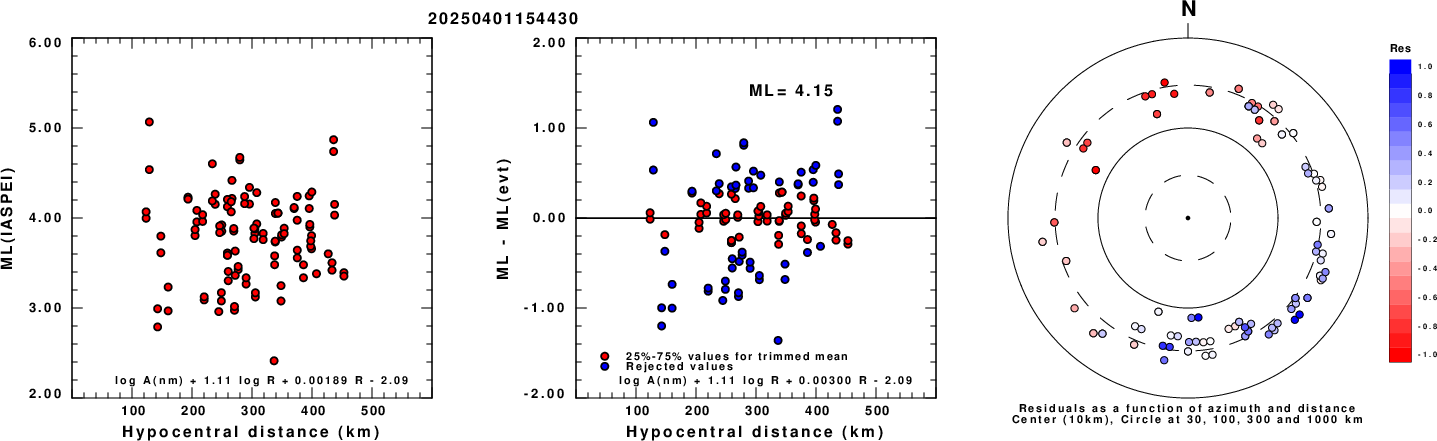
Left: ML computed using the IASPEI formula for Horizontal components. Center: ML residuals computed using a modified IASPEI formula that accounts for path specific attenuation; the values used for the trimmed mean are indicated. The ML relation used for each figure is given at the bottom of each plot.
Right: Residuals from new relation as a function of distance and azimuth.
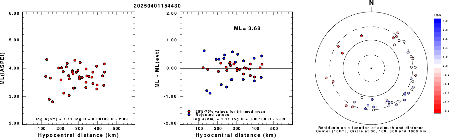
Left: ML computed using the IASPEI formula for Vertical components (research). Center: ML residuals computed using a modified IASPEI formula that accounts for path specific attenuation; the values used for the trimmed mean are indicated. The ML relation used for each figure is given at the bottom of each plot.
Right: Residuals from new relation as a function of distance and azimuth.
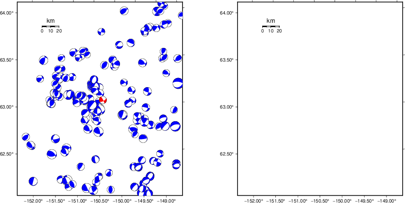 |
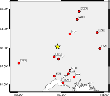
The focal mechanism was determined using broadband seismic waveforms. The location of the event (star) and the stations used for (red) the waveform inversion are shown in the next figure.
|
|
|
The program wvfgrd96 was used with good traces observed at short distance to determine the focal mechanism, depth and seismic moment. This technique requires a high quality signal and well determined velocity model for the Green's functions. To the extent that these are the quality data, this type of mechanism should be preferred over the radiation pattern technique which requires the separate step of defining the pressure and tension quadrants and the correct strike.
The observed and predicted traces are filtered using the following gsac commands:
cut o DIST/3.5 -40 o DIST/3.5 +50
rtr
taper w 0.1
hp c 0.03 n 3
lp c 0.08 n 3
The results of this grid search are as follow:
           DEPTH  STK   DIP  RAKE   MW    FIT
WVFGRD96    2.0   150    65   -35   3.01 0.2750
WVFGRD96    4.0   345    70    30   3.10 0.2976
WVFGRD96    6.0   165    55    20   3.14 0.3305
WVFGRD96    8.0   165    55    20   3.21 0.3532
WVFGRD96   10.0   160    60    10   3.23 0.3600
WVFGRD96   12.0   340    80    30   3.28 0.3583
WVFGRD96   14.0   335    90    30   3.30 0.3568
WVFGRD96   16.0   155    85   -30   3.32 0.3529
WVFGRD96   18.0   335    90    30   3.34 0.3392
WVFGRD96   20.0   240    55   -25   3.39 0.3416
WVFGRD96   22.0   240    50   -20   3.42 0.3517
WVFGRD96   24.0   240    50   -15   3.44 0.3638
WVFGRD96   26.0   245    55   -15   3.46 0.3786
WVFGRD96   28.0   245    60   -15   3.48 0.3956
WVFGRD96   30.0   245    65   -15   3.50 0.4120
WVFGRD96   32.0   245    65    -5   3.51 0.4271
WVFGRD96   34.0   245    65    -5   3.54 0.4443
WVFGRD96   36.0   245    70    -5   3.56 0.4557
WVFGRD96   38.0   245    80   -10   3.58 0.4634
WVFGRD96   40.0   240    70   -15   3.65 0.4907
WVFGRD96   42.0   245    65    -5   3.67 0.4914
WVFGRD96   44.0   240    70   -10   3.69 0.4933
WVFGRD96   46.0   245    65    -5   3.71 0.4959
WVFGRD96   48.0   245    65    -5   3.73 0.4980
WVFGRD96   50.0   245    65    -5   3.75 0.5027
WVFGRD96   52.0   245    70    -5   3.75 0.5082
WVFGRD96   54.0   245    70    -5   3.76 0.5144
WVFGRD96   56.0   245    70    -5   3.78 0.5229
WVFGRD96   58.0   245    70     0   3.79 0.5297
WVFGRD96   60.0   245    85   -15   3.77 0.5361
WVFGRD96   62.0   245    85   -15   3.78 0.5433
WVFGRD96   64.0   245    75     0   3.81 0.5501
WVFGRD96   66.0   245    90   -15   3.78 0.5596
WVFGRD96   68.0    65    75    15   3.77 0.5689
WVFGRD96   70.0    65    75    15   3.77 0.5775
WVFGRD96   72.0    65    75    15   3.77 0.5861
WVFGRD96   74.0    65    70    15   3.78 0.5944
WVFGRD96   76.0    65    70    15   3.78 0.6012
WVFGRD96   78.0    65    70    15   3.78 0.6074
WVFGRD96   80.0    65    75    10   3.79 0.6127
WVFGRD96   82.0    65    70    10   3.79 0.6194
WVFGRD96   84.0    65    70    10   3.79 0.6248
WVFGRD96   86.0    65    70    10   3.80 0.6299
WVFGRD96   88.0    65    70    10   3.80 0.6322
WVFGRD96   90.0    65    70    10   3.80 0.6362
WVFGRD96   92.0    65    70    10   3.81 0.6393
WVFGRD96   94.0    65    70    10   3.81 0.6420
WVFGRD96   96.0    65    70     5   3.82 0.6446
WVFGRD96   98.0    65    70     5   3.82 0.6461
WVFGRD96  100.0    65    70     5   3.82 0.6483
WVFGRD96  102.0    65    70     5   3.82 0.6494
WVFGRD96  104.0    65    70     5   3.83 0.6488
WVFGRD96  106.0    65    70     5   3.83 0.6510
WVFGRD96  108.0    65    65     5   3.82 0.6507
WVFGRD96  110.0    65    65     5   3.83 0.6506
WVFGRD96  112.0    65    65     5   3.83 0.6510
WVFGRD96  114.0    65    65     5   3.83 0.6507
WVFGRD96  116.0    65    65     5   3.83 0.6507
WVFGRD96  118.0    65    60    10   3.82 0.6499
WVFGRD96  120.0    65    65     5   3.84 0.6482
WVFGRD96  122.0    65    60    10   3.83 0.6486
WVFGRD96  124.0    65    60    10   3.83 0.6468
WVFGRD96  126.0    65    60    10   3.83 0.6465
WVFGRD96  128.0    65    60    10   3.83 0.6448
WVFGRD96  130.0    65    60    10   3.84 0.6442
WVFGRD96  132.0    65    60    10   3.84 0.6430
WVFGRD96  134.0    65    60    10   3.84 0.6408
WVFGRD96  136.0    65    60    10   3.84 0.6402
WVFGRD96  138.0    65    60    10   3.84 0.6386
WVFGRD96  140.0    65    60    10   3.85 0.6375
WVFGRD96  142.0    65    55    15   3.84 0.6358
WVFGRD96  144.0    65    55    15   3.84 0.6353
WVFGRD96  146.0    65    55    15   3.85 0.6332
WVFGRD96  148.0    65    55    15   3.85 0.6322
The best solution is
WVFGRD96 112.0 65 65 5 3.83 0.6510
The mechanism corresponding to the best fit is
|
|
|
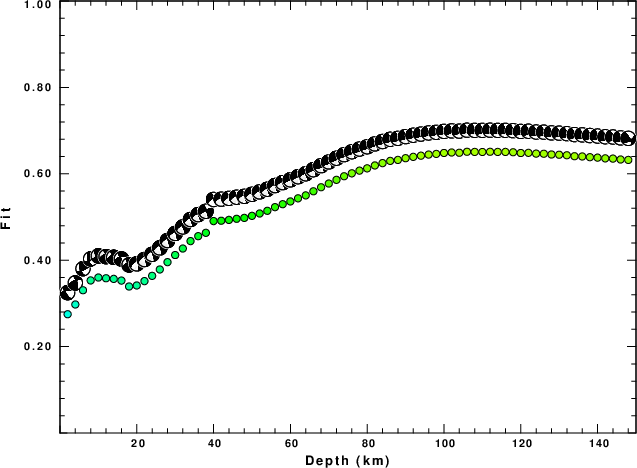
The best fit as a function of depth is given in the following figure:
|
|
|
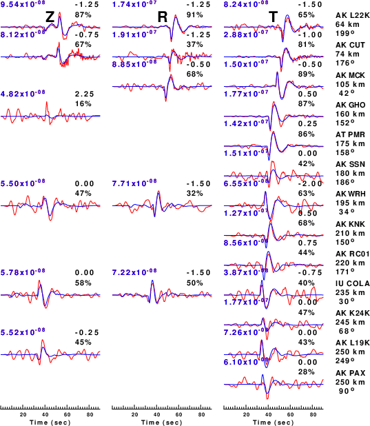
The comparison of the observed and predicted waveforms is given in the next figure. The red traces are the observed and the blue are the predicted. Each observed-predicted component is plotted to the same scale and peak amplitudes are indicated by the numbers to the left of each trace. A pair of numbers is given in black at the right of each predicted traces. The upper number it the time shift required for maximum correlation between the observed and predicted traces. This time shift is required because the synthetics are not computed at exactly the same distance as the observed, the velocity model used in the predictions may not be perfect and the epicentral parameters may be be off. A positive time shift indicates that the prediction is too fast and should be delayed to match the observed trace (shift to the right in this figure). A negative value indicates that the prediction is too slow. The lower number gives the percentage of variance reduction to characterize the individual goodness of fit (100% indicates a perfect fit).
The bandpass filter used in the processing and for the display was
cut o DIST/3.5 -40 o DIST/3.5 +50
rtr
taper w 0.1
hp c 0.03 n 3
lp c 0.08 n 3
|
| Figure 3. Waveform comparison for selected depth. Red: observed; Blue - predicted. The time shift with respect to the model prediction is indicated. The percent of fit is also indicated. The time scale is relative to the first trace sample. |
|
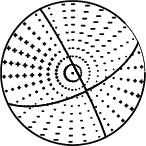
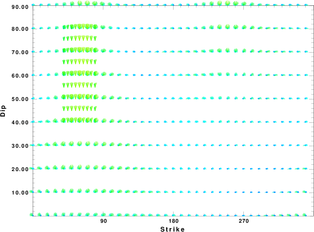
| Focal mechanism sensitivity at the preferred depth. The red color indicates a very good fit to the waveforms. Each solution is plotted as a vector at a given value of strike and dip with the angle of the vector representing the rake angle, measured, with respect to the upward vertical (N) in the figure. |
A check on the assumed source location is possible by looking at the time shifts between the observed and predicted traces. The time shifts for waveform matching arise for several reasons:
Time_shift = A + B cos Azimuth + C Sin Azimuth
The time shifts for this inversion lead to the next figure:
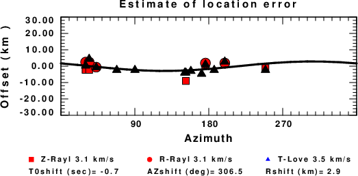
The derived shift in origin time and epicentral coordinates are given at the bottom of the figure.
The WUS.model used for the waveform synthetic seismograms and for the surface wave eigenfunctions and dispersion is as follows (The format is in the model96 format of Computer Programs in Seismology).
MODEL.01
Model after     8 iterations
ISOTROPIC
KGS
FLAT EARTH
1-D
CONSTANT VELOCITY
LINE08
LINE09
LINE10
LINE11
      H(KM)   VP(KM/S)   VS(KM/S) RHO(GM/CC)         QP         QS       ETAP       ETAS      FREFP      FREFS
     1.9000     3.4065     2.0089     2.2150  0.302E-02  0.679E-02   0.00       0.00       1.00       1.00
     6.1000     5.5445     3.2953     2.6089  0.349E-02  0.784E-02   0.00       0.00       1.00       1.00
    13.0000     6.2708     3.7396     2.7812  0.212E-02  0.476E-02   0.00       0.00       1.00       1.00
    19.0000     6.4075     3.7680     2.8223  0.111E-02  0.249E-02   0.00       0.00       1.00       1.00
     0.0000     7.9000     4.6200     3.2760  0.164E-10  0.370E-10   0.00       0.00       1.00       1.00