Location
Location ANSS
The ANSS event ID is us7000pfbs and the event page is at
https://earthquake.usgs.gov/earthquakes/eventpage/us7000pfbs/executive.
2025/02/21 21:26:33 49.631 -123.534 10.0 4.8 B.C., Canada
Focal Mechanism
 USGS/SLU Moment Tensor Solution
 ENS  2025/02/21 21:26:33:0  49.63 -123.53  10.0 4.8 B.C., Canada

 Stations used:
   C8.BCOV CN.BBB CN.CBB CN.CLRS CN.EDB CN.FHBB CN.GDR CN.GHNB
   CN.GOBB CN.HOLB CN.HOPB CN.LLLB CN.NLLB CN.OZB CN.PABB
   CN.PGC CN.PHC CN.PTRF CN.QEPB CN.SYMB CN.TOFB CN.TXDB
   CN.VDEB CN.VGZ CN.WOSB CN.WSLR PQ.ALBHB PQ.DAOB PQ.HAKB
   RE.GRCO2 UO.GROV UO.GRSDL UO.MINN UO.MONKS UO.NBFR UO.NECAN
   UO.SADL UO.SKAN UO.STONY UO.TRASK UO.TRIPT UO.VERN UO.WIKI
   US.NEW US.NLWA UW.ABER UW.BDGR UW.BHAM UW.BHCR UW.BLOB
   UW.BOIS UW.BUCKS UW.CBS UW.CCRK UW.CDF UW.CHIMA UW.CORE
   UW.COYL UW.CROWN UW.CVILL UW.DART UW.DAVN UW.DDRF UW.DEAL
   UW.DONK UW.DOORS UW.DOSE UW.DOTY UW.DY2 UW.EPH2 UW.EQUIL
   UW.ETW UW.FISH2 UW.FORK UW.GBB UW.GOBBL UW.GPW UW.H2O
   UW.HDW UW.HERD UW.HOPR UW.HOQUI UW.HTW UW.INGAL UW.KALA
   UW.KTSAP UW.LEID UW.LMONT UW.LOPEZ UW.LRIV UW.MBW2 UW.MDW
   UW.METAL UW.MONTE UW.MOODY UW.MULN UW.NIKE UW.OD2 UW.ODUC
   UW.OHOH UW.OLGA UW.OLQN UW.OMAK UW.OQNOB UW.OSQM UW.OSR
   UW.OT3 UW.OTR UW.PAN4H UW.PASS UW.RNWY UW.RPW2 UW.RVSD
   UW.SALO UW.SAW UW.SAXON UW.SHUK UW.SKAMO UW.SKOKO UW.SLDQ
   UW.SLF UW.SNAG UW.TNSKT UW.TOUT UW.TURTL UW.TWISP UW.WA2
   UW.WAT2 UW.WINDI UW.WOLL UW.WYNO

 Filtering commands used:
   cut o DIST/3.3 -40 o DIST/3.3 +50
   rtr
   taper w 0.1
   hp c 0.03 n 3
   lp c 0.07 n 3

 Best Fitting Double Couple
  Mo = 1.27e+23 dyne-cm
  Mw = 4.67
  Z  = 15 km
  Plane   Strike  Dip  Rake
   NP1      279    76   154
   NP2       15    65    15
  Principal Axes:
   Axis    Value   Plunge  Azimuth
    T   1.27e+23     28     235
    N   0.00e+00     61      73
    P  -1.27e+23      8     329

 Moment Tensor: (dyne-cm)
    Component   Value
       Mxx    -5.74e+22
       Mxy     1.03e+23
       Mxz    -4.47e+22
       Myy     3.22e+22
       Myz    -3.39e+22
       Mzz     2.52e+22


                     -------------#
                   ---------------#####
              -- P ----------------#######
             ---   ----------------########
           -------------------------#########
          --------------------------##########
         ---------------------------###########
        ----------------------------############
        ---------------------------#############
       #########################---##############
       ############################-----#########
       ###########################-----------####
       ###########################--------------#
        #########################---------------
        ######   ################---------------
         ##### T ###############---------------
          ####   ##############---------------
           ###################---------------
             ################--------------
              #############---------------
                 #########-------------
                     ###-----------


 Global CMT Convention Moment Tensor:
      R          T          P
  2.52e+22  -4.47e+22   3.39e+22
 -4.47e+22  -5.74e+22  -1.03e+23
  3.39e+22  -1.03e+23   3.22e+22


Details of the solution is found at

http://www.eas.slu.edu/eqc/eqc_mt/MECH.NA/20250221212633/index.html
|
Preferred Solution
The preferred solution from an analysis of the surface-wave spectral amplitude radiation pattern, waveform inversion or first motion observations is
      STK = 15
      DIP = 65
     RAKE = 15
       MW = 4.67
       HS = 15.0
The NDK file is 20250221212633.ndk
The waveform inversion is preferred.
Moment Tensor Comparison
The following compares this source inversion to those provided by others. The purpose is to look for major differences and also to note slight differences that might be inherent to the processing procedure. For completeness the USGS/SLU solution is repeated from above.
| SLU |
USGSW |
 USGS/SLU Moment Tensor Solution
 ENS  2025/02/21 21:26:33:0  49.63 -123.53  10.0 4.8 B.C., Canada

 Stations used:
   C8.BCOV CN.BBB CN.CBB CN.CLRS CN.EDB CN.FHBB CN.GDR CN.GHNB
   CN.GOBB CN.HOLB CN.HOPB CN.LLLB CN.NLLB CN.OZB CN.PABB
   CN.PGC CN.PHC CN.PTRF CN.QEPB CN.SYMB CN.TOFB CN.TXDB
   CN.VDEB CN.VGZ CN.WOSB CN.WSLR PQ.ALBHB PQ.DAOB PQ.HAKB
   RE.GRCO2 UO.GROV UO.GRSDL UO.MINN UO.MONKS UO.NBFR UO.NECAN
   UO.SADL UO.SKAN UO.STONY UO.TRASK UO.TRIPT UO.VERN UO.WIKI
   US.NEW US.NLWA UW.ABER UW.BDGR UW.BHAM UW.BHCR UW.BLOB
   UW.BOIS UW.BUCKS UW.CBS UW.CCRK UW.CDF UW.CHIMA UW.CORE
   UW.COYL UW.CROWN UW.CVILL UW.DART UW.DAVN UW.DDRF UW.DEAL
   UW.DONK UW.DOORS UW.DOSE UW.DOTY UW.DY2 UW.EPH2 UW.EQUIL
   UW.ETW UW.FISH2 UW.FORK UW.GBB UW.GOBBL UW.GPW UW.H2O
   UW.HDW UW.HERD UW.HOPR UW.HOQUI UW.HTW UW.INGAL UW.KALA
   UW.KTSAP UW.LEID UW.LMONT UW.LOPEZ UW.LRIV UW.MBW2 UW.MDW
   UW.METAL UW.MONTE UW.MOODY UW.MULN UW.NIKE UW.OD2 UW.ODUC
   UW.OHOH UW.OLGA UW.OLQN UW.OMAK UW.OQNOB UW.OSQM UW.OSR
   UW.OT3 UW.OTR UW.PAN4H UW.PASS UW.RNWY UW.RPW2 UW.RVSD
   UW.SALO UW.SAW UW.SAXON UW.SHUK UW.SKAMO UW.SKOKO UW.SLDQ
   UW.SLF UW.SNAG UW.TNSKT UW.TOUT UW.TURTL UW.TWISP UW.WA2
   UW.WAT2 UW.WINDI UW.WOLL UW.WYNO

 Filtering commands used:
   cut o DIST/3.3 -40 o DIST/3.3 +50
   rtr
   taper w 0.1
   hp c 0.03 n 3
   lp c 0.07 n 3

 Best Fitting Double Couple
  Mo = 1.27e+23 dyne-cm
  Mw = 4.67
  Z  = 15 km
  Plane   Strike  Dip  Rake
   NP1      279    76   154
   NP2       15    65    15
  Principal Axes:
   Axis    Value   Plunge  Azimuth
    T   1.27e+23     28     235
    N   0.00e+00     61      73
    P  -1.27e+23      8     329

 Moment Tensor: (dyne-cm)
    Component   Value
       Mxx    -5.74e+22
       Mxy     1.03e+23
       Mxz    -4.47e+22
       Myy     3.22e+22
       Myz    -3.39e+22
       Mzz     2.52e+22


                     -------------#
                   ---------------#####
              -- P ----------------#######
             ---   ----------------########
           -------------------------#########
          --------------------------##########
         ---------------------------###########
        ----------------------------############
        ---------------------------#############
       #########################---##############
       ############################-----#########
       ###########################-----------####
       ###########################--------------#
        #########################---------------
        ######   ################---------------
         ##### T ###############---------------
          ####   ##############---------------
           ###################---------------
             ################--------------
              #############---------------
                 #########-------------
                     ###-----------


 Global CMT Convention Moment Tensor:
      R          T          P
  2.52e+22  -4.47e+22   3.39e+22
 -4.47e+22  -5.74e+22  -1.03e+23
  3.39e+22  -1.03e+23   3.22e+22


Details of the solution is found at

http://www.eas.slu.edu/eqc/eqc_mt/MECH.NA/20250221212633/index.html
|
W-phase Moment Tensor (Mww)
Moment
2.050e+16 N-m
Magnitude
4.81 Mww
Depth
19.5 km
Percent DC
88%
Half Duration
0.50 s
Catalog
US
Data Source
US
Contributor
US
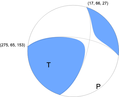
Nodal Planes
Plane Strike Dip Rake
NP1 275 65 153
NP2 17 66 27
Principal Axes
Axis Value Plunge Azimuth
T 2.110e+16 36 237
N -0.126e+16 54 56
P -1.984e+16 0 146
|
Magnitudes
Given the availability of digital waveforms for determination of the moment tensor, this section documents the added processing leading to mLg, if appropriate to the region, and ML by application of the respective IASPEI formulae. As a research study, the linear distance term of the IASPEI formula
for ML is adjusted to remove a linear distance trend in residuals to give a regionally defined ML. The defined ML uses horizontal component recordings, but the same procedure is applied to the vertical components since there may be some interest in vertical component ground motions. Residual plots versus distance may indicate interesting features of ground motion scaling in some distance ranges. A residual plot of the regionalized magnitude is given as a function of distance and azimuth, since data sets may transcend different wave propagation provinces.
ML Magnitude
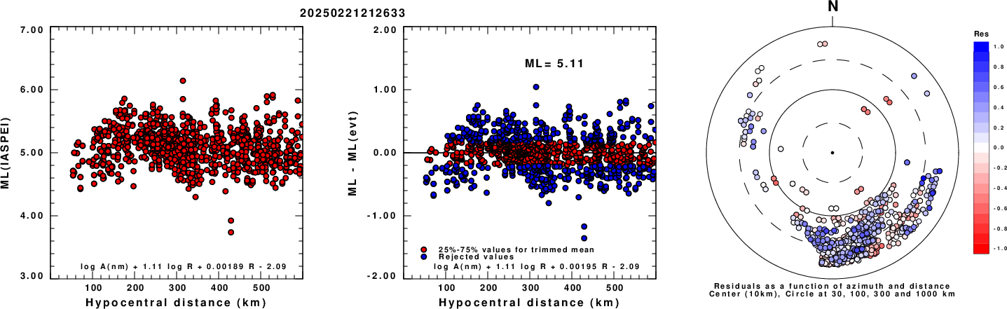
Left: ML computed using the IASPEI formula for Horizontal components. Center: ML residuals computed using a modified IASPEI formula that accounts for path specific attenuation; the values used for the trimmed mean are indicated. The ML relation used for each figure is given at the bottom of each plot.
Right: Residuals from new relation as a function of distance and azimuth.
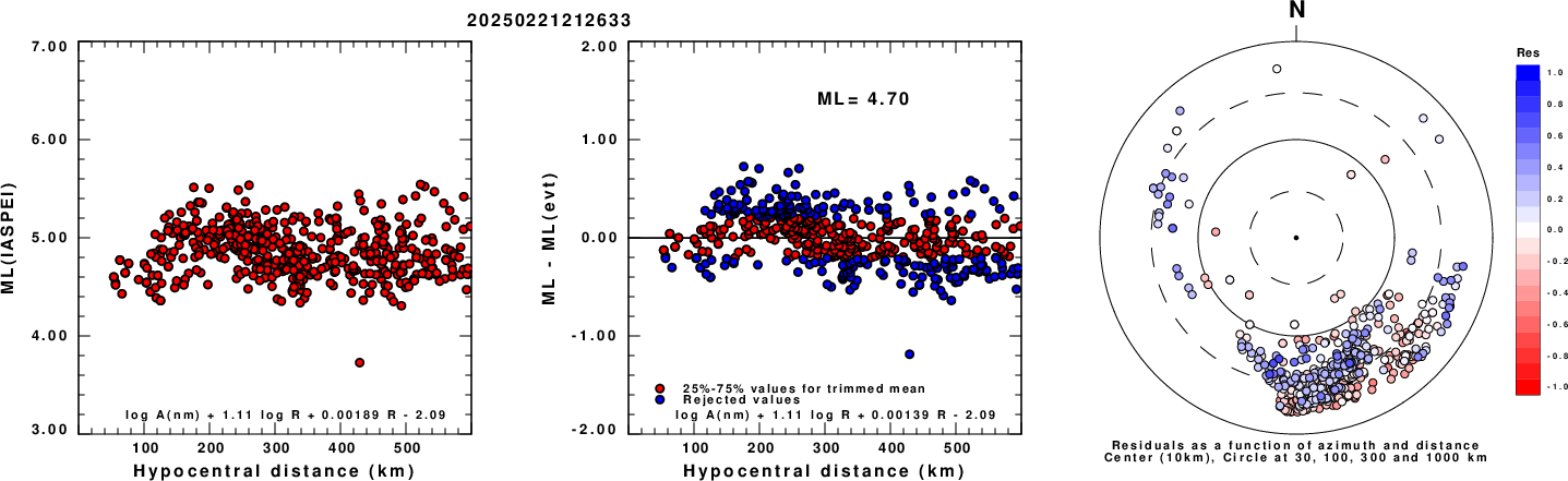
Left: ML computed using the IASPEI formula for Vertical components (research). Center: ML residuals computed using a modified IASPEI formula that accounts for path specific attenuation; the values used for the trimmed mean are indicated. The ML relation used for each figure is given at the bottom of each plot.
Right: Residuals from new relation as a function of distance and azimuth.
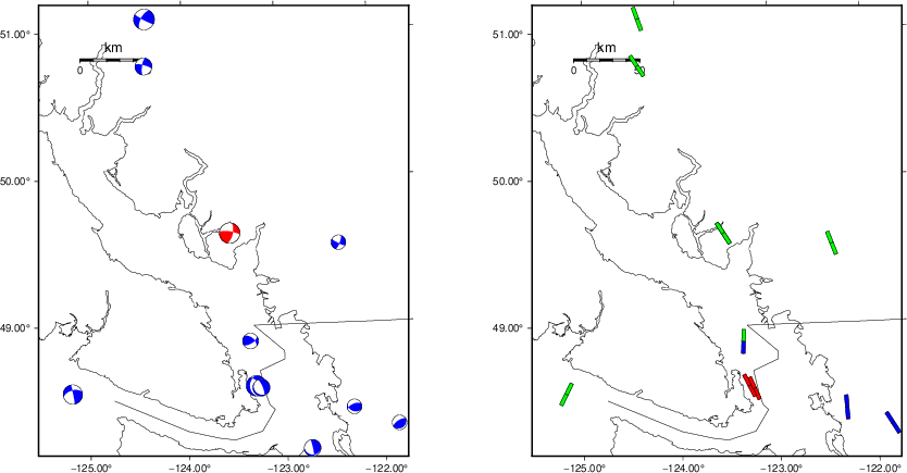
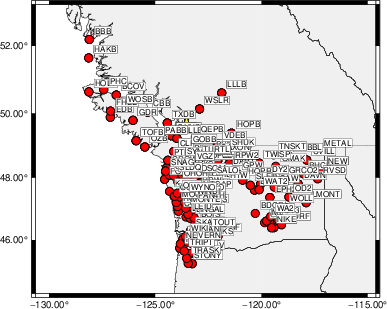
Context
The left panel of the next figure presents the focal mechanism for this earthquake (red) in the context of other nearby events (blue) in the SLU Moment Tensor Catalog. The right panel shows the inferred direction of maximum compressive stress and the type of faulting (green is strike-slip, red is normal, blue is thrust; oblique is shown by a combination of colors). Thus context plot is useful for assessing the appropriateness of the moment tensor of this event.
Waveform Inversion using wvfgrd96
The focal mechanism was determined using broadband seismic waveforms. The location of the event (star) and the
stations used for (red) the waveform inversion are shown in the next figure.
|
|
Location of broadband stations used for waveform inversion
|
The program wvfgrd96 was used with good traces observed at short distance to determine the focal mechanism, depth and seismic moment. This technique requires a high quality signal and well determined velocity model for the Green's functions. To the extent that these are the quality data, this type of mechanism should be preferred over the radiation pattern technique which requires the separate step of defining the pressure and tension quadrants and the correct strike.
The observed and predicted traces are filtered using the following gsac commands:
cut o DIST/3.3 -40 o DIST/3.3 +50
rtr
taper w 0.1
hp c 0.03 n 3
lp c 0.07 n 3
The results of this grid search are as follow:
           DEPTH  STK   DIP  RAKE   MW    FIT
WVFGRD96    1.0   195    85     5   4.21 0.2889
WVFGRD96    2.0    15    90     0   4.32 0.3725
WVFGRD96    3.0    10    70   -10   4.38 0.3997
WVFGRD96    4.0    10    65   -15   4.43 0.4255
WVFGRD96    5.0    10    55    -5   4.47 0.4579
WVFGRD96    6.0    10    55    -5   4.49 0.4946
WVFGRD96    7.0    10    60    -5   4.51 0.5295
WVFGRD96    8.0    15    55    15   4.57 0.5624
WVFGRD96    9.0    15    55    15   4.59 0.5957
WVFGRD96   10.0    15    60    20   4.61 0.6227
WVFGRD96   11.0    15    60    20   4.62 0.6456
WVFGRD96   12.0    15    60    20   4.64 0.6618
WVFGRD96   13.0    15    60    20   4.65 0.6719
WVFGRD96   14.0    15    65    20   4.66 0.6785
WVFGRD96   15.0    15    65    15   4.67 0.6815
WVFGRD96   16.0    15    65    15   4.68 0.6811
WVFGRD96   17.0    15    65    15   4.69 0.6778
WVFGRD96   18.0    15    65    15   4.70 0.6719
WVFGRD96   19.0    15    65    15   4.71 0.6640
WVFGRD96   20.0    15    65    15   4.71 0.6544
WVFGRD96   21.0    15    65    15   4.72 0.6433
WVFGRD96   22.0    15    65    15   4.73 0.6314
WVFGRD96   23.0    15    65    15   4.73 0.6185
WVFGRD96   24.0    15    65    15   4.74 0.6052
WVFGRD96   25.0    15    65    15   4.75 0.5915
WVFGRD96   26.0    15    65    15   4.75 0.5776
WVFGRD96   27.0    15    65    15   4.76 0.5635
WVFGRD96   28.0    15    65    15   4.76 0.5496
WVFGRD96   29.0    15    65    15   4.77 0.5357
The best solution is
WVFGRD96 15.0 15 65 15 4.67 0.6815
The mechanism corresponding to the best fit is
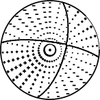
|
|
Figure 1. Waveform inversion focal mechanism
|
The best fit as a function of depth is given in the following figure:
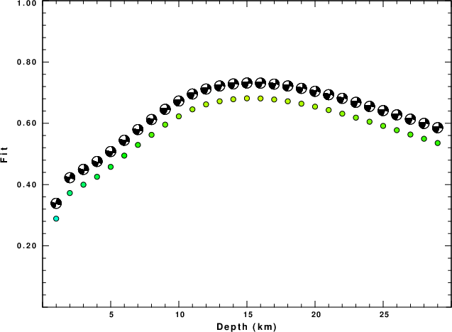
|
|
Figure 2. Depth sensitivity for waveform mechanism
|
The comparison of the observed and predicted waveforms is given in the next figure. The red traces are the observed and the blue are the predicted.
Each observed-predicted component is plotted to the same scale and peak amplitudes are indicated by the numbers to the left of each trace. A pair of numbers is given in black at the right of each predicted traces. The upper number it the time shift required for maximum correlation between the observed and predicted traces. This time shift is required because the synthetics are not computed at exactly the same distance as the observed, the velocity model used in the predictions may not be perfect and the epicentral parameters may be be off.
A positive time shift indicates that the prediction is too fast and should be delayed to match the observed trace (shift to the right in this figure). A negative value indicates that the prediction is too slow. The lower number gives the percentage of variance reduction to characterize the individual goodness of fit (100% indicates a perfect fit).
The bandpass filter used in the processing and for the display was
cut o DIST/3.3 -40 o DIST/3.3 +50
rtr
taper w 0.1
hp c 0.03 n 3
lp c 0.07 n 3

|
|
Figure 3. Waveform comparison for selected depth. Red: observed; Blue - predicted. The time shift with respect to the model prediction is indicated. The percent of fit is also indicated. The time scale is relative to the first trace sample.
|
|
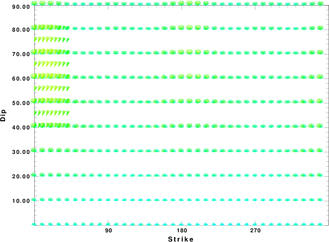
|
Focal mechanism sensitivity at the preferred depth. The red color indicates a very good fit to the waveforms.
Each solution is plotted as a vector at a given value of strike and dip with the angle of the vector representing the rake angle, measured, with respect to the upward vertical (N) in the figure.
|
A check on the assumed source location is possible by looking at the time shifts between the observed and predicted traces. The time shifts for waveform matching arise for several reasons:
- The origin time and epicentral distance are incorrect
- The velocity model used for the inversion is incorrect
- The velocity model used to define the P-arrival time is not the
same as the velocity model used for the waveform inversion
(assuming that the initial trace alignment is based on the
P arrival time)
Assuming only a mislocation, the time shifts are fit to a functional form:
Time_shift = A + B cos Azimuth + C Sin Azimuth
The time shifts for this inversion lead to the next figure:
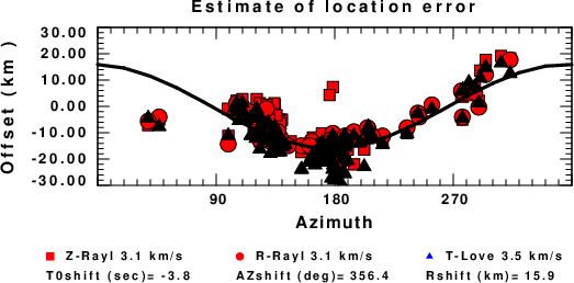
The derived shift in origin time and epicentral coordinates are given at the bottom of the figure.
Velocity Model
The WUS.model used for the waveform synthetic seismograms and for the surface wave eigenfunctions and dispersion is as follows
(The format is in the model96 format of Computer Programs in Seismology).
MODEL.01
Model after     8 iterations
ISOTROPIC
KGS
FLAT EARTH
1-D
CONSTANT VELOCITY
LINE08
LINE09
LINE10
LINE11
      H(KM)   VP(KM/S)   VS(KM/S) RHO(GM/CC)         QP         QS       ETAP       ETAS      FREFP      FREFS
     1.9000     3.4065     2.0089     2.2150  0.302E-02  0.679E-02   0.00       0.00       1.00       1.00
     6.1000     5.5445     3.2953     2.6089  0.349E-02  0.784E-02   0.00       0.00       1.00       1.00
    13.0000     6.2708     3.7396     2.7812  0.212E-02  0.476E-02   0.00       0.00       1.00       1.00
    19.0000     6.4075     3.7680     2.8223  0.111E-02  0.249E-02   0.00       0.00       1.00       1.00
     0.0000     7.9000     4.6200     3.2760  0.164E-10  0.370E-10   0.00       0.00       1.00       1.00
Last Changed Fri Feb 21 17:02:26 CST 2025