Location
Location ANSS
The ANSS event ID is ak024gb66mji and the event page is at
https://earthquake.usgs.gov/earthquakes/eventpage/ak024gb66mji/executive.
2024/12/20 04:03:22 60.357 -152.294 84.7 4.5 Alaska
Focal Mechanism
USGS/SLU Moment Tensor Solution
ENS 2024/12/20 04:03:22:0 60.36 -152.29 84.7 4.5 Alaska
Stations used:
AK.BRLK AK.CAPN AK.CUT AK.FIRE AK.GHO AK.HOM AK.L19K
AK.L22K AK.M20K AK.N18K AK.N19K AK.O18K AK.O19K AK.P17K
AK.RC01 AK.SAW AK.SLK AK.SSN AK.SWD AT.PMR AV.ACH AV.RED
AV.STLK II.KDAK
Filtering commands used:
cut o DIST/3.3 -50 o DIST/3.3 +40
rtr
taper w 0.1
hp c 0.03 n 3
lp c 0.07 n 3
br c 0.12 0.25 n 4 p 2
Best Fitting Double Couple
Mo = 1.19e+23 dyne-cm
Mw = 4.65
Z = 112 km
Plane Strike Dip Rake
NP1 50 70 35
NP2 307 57 156
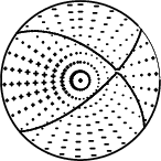
Principal Axes:
Axis Value Plunge Azimuth
T 1.19e+23 39 272
N 0.00e+00 50 76
P -1.19e+23 8 176
Moment Tensor: (dyne-cm)
Component Value
Mxx -1.16e+23
Mxy 5.69e+21
Mxz 1.86e+22
Myy 7.20e+22
Myz -5.91e+22
Mzz 4.38e+22
--------------
----------------------
----------------------------
------------------------------
###########----------------------#
#################----------------###
#####################------------#####
#########################--------#######
###########################----#########
####### ####################-###########
####### T ###################---##########
####### ##################-----#########
##########################---------#######
######################-------------#####
####################---------------#####
################-------------------###
############----------------------##
#######---------------------------
------------------------------
----------------------------
----------- --------
------- P ----
Global CMT Convention Moment Tensor:
R T P
4.38e+22 1.86e+22 5.91e+22
1.86e+22 -1.16e+23 -5.69e+21
5.91e+22 -5.69e+21 7.20e+22
Details of the solution is found at
http://www.eas.slu.edu/eqc/eqc_mt/MECH.NA/20241220040322/index.html
|
Preferred Solution
The preferred solution from an analysis of the surface-wave spectral amplitude radiation pattern, waveform inversion or first motion observations is
      STK = 50
      DIP = 70
     RAKE = 35
       MW = 4.65
       HS = 112.0
The NDK file is 20241220040322.ndk
The waveform inversion is preferred.
Magnitudes
Given the availability of digital waveforms for determination of the moment tensor, this section documents the added processing leading to mLg, if appropriate to the region, and ML by application of the respective IASPEI formulae. As a research study, the linear distance term of the IASPEI formula
for ML is adjusted to remove a linear distance trend in residuals to give a regionally defined ML. The defined ML uses horizontal component recordings, but the same procedure is applied to the vertical components since there may be some interest in vertical component ground motions. Residual plots versus distance may indicate interesting features of ground motion scaling in some distance ranges. A residual plot of the regionalized magnitude is given as a function of distance and azimuth, since data sets may transcend different wave propagation provinces.
ML Magnitude
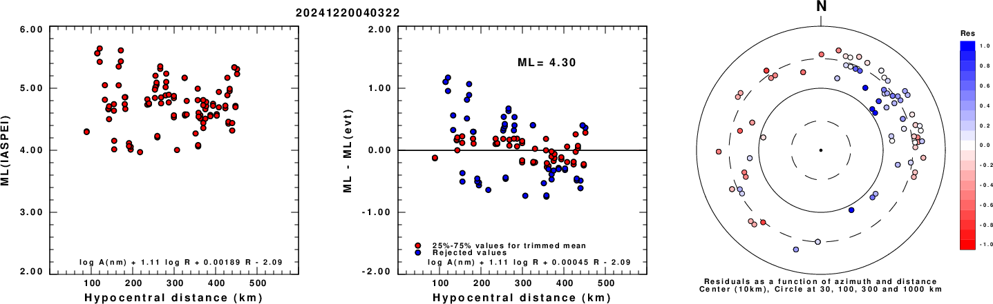
Left: ML computed using the IASPEI formula for Horizontal components. Center: ML residuals computed using a modified IASPEI formula that accounts for path specific attenuation; the values used for the trimmed mean are indicated. The ML relation used for each figure is given at the bottom of each plot.
Right: Residuals from new relation as a function of distance and azimuth.
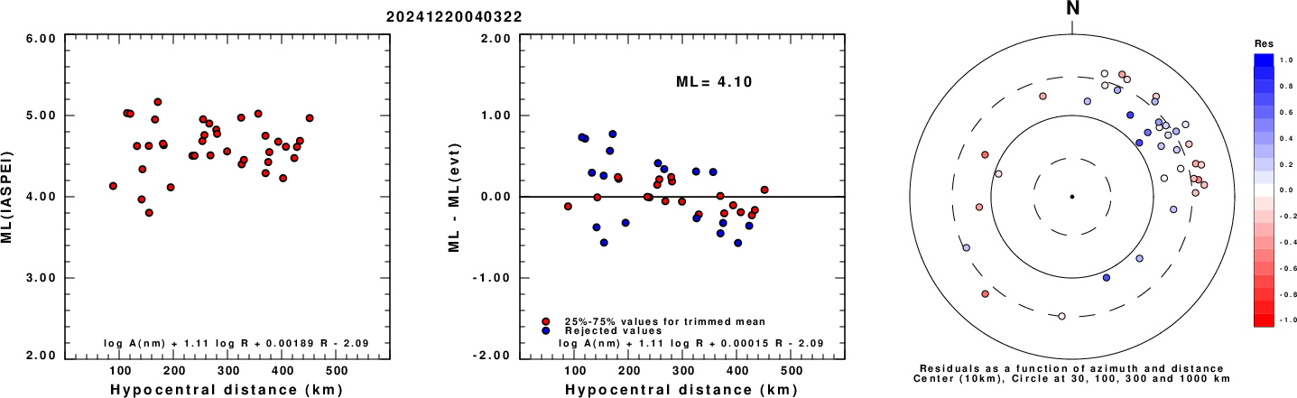
Left: ML computed using the IASPEI formula for Vertical components (research). Center: ML residuals computed using a modified IASPEI formula that accounts for path specific attenuation; the values used for the trimmed mean are indicated. The ML relation used for each figure is given at the bottom of each plot.
Right: Residuals from new relation as a function of distance and azimuth.
Context
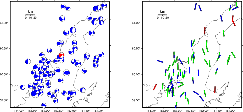
The left panel of the next figure presents the focal mechanism for this earthquake (red) in the context of other nearby events (blue) in the SLU Moment Tensor Catalog. The right panel shows the inferred direction of maximum compressive stress and the type of faulting (green is strike-slip, red is normal, blue is thrust; oblique is shown by a combination of colors). Thus context plot is useful for assessing the appropriateness of the moment tensor of this event.
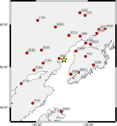
Waveform Inversion using wvfgrd96
The focal mechanism was determined using broadband seismic waveforms. The location of the event (star) and the
stations used for (red) the waveform inversion are shown in the next figure.
|
|
Location of broadband stations used for waveform inversion
|
The program wvfgrd96 was used with good traces observed at short distance to determine the focal mechanism, depth and seismic moment. This technique requires a high quality signal and well determined velocity model for the Green's functions. To the extent that these are the quality data, this type of mechanism should be preferred over the radiation pattern technique which requires the separate step of defining the pressure and tension quadrants and the correct strike.
The observed and predicted traces are filtered using the following gsac commands:
cut o DIST/3.3 -50 o DIST/3.3 +40
rtr
taper w 0.1
hp c 0.03 n 3
lp c 0.07 n 3
br c 0.12 0.25 n 4 p 2
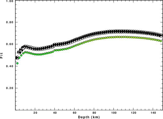
The results of this grid search are as follow:
           DEPTH  STK   DIP  RAKE   MW    FIT
WVFGRD96    2.0    55    65    30   3.94 0.4263
WVFGRD96    4.0   235    65    25   4.00 0.4775
WVFGRD96    6.0   230    75    15   4.02 0.4990
WVFGRD96    8.0   225    65   -20   4.07 0.5176
WVFGRD96   10.0   225    70   -15   4.09 0.5273
WVFGRD96   12.0   225    75   -10   4.11 0.5255
WVFGRD96   14.0   225    80     5   4.12 0.5214
WVFGRD96   16.0   225    80     5   4.14 0.5170
WVFGRD96   18.0   225    80     5   4.16 0.5116
WVFGRD96   20.0    45    80     5   4.18 0.5084
WVFGRD96   22.0    45    80     5   4.20 0.5069
WVFGRD96   24.0    45    80    10   4.22 0.5066
WVFGRD96   26.0    45    80    10   4.23 0.5075
WVFGRD96   28.0    45    80    10   4.25 0.5102
WVFGRD96   30.0    45    80    10   4.27 0.5137
WVFGRD96   32.0    45    80    10   4.29 0.5178
WVFGRD96   34.0    45    85    10   4.31 0.5216
WVFGRD96   36.0    45    85    10   4.34 0.5256
WVFGRD96   38.0    45    85    10   4.37 0.5313
WVFGRD96   40.0    45    80    10   4.41 0.5438
WVFGRD96   42.0    45    80    10   4.43 0.5458
WVFGRD96   44.0    45    80    15   4.45 0.5471
WVFGRD96   46.0    45    80    15   4.46 0.5494
WVFGRD96   48.0    45    80    15   4.48 0.5523
WVFGRD96   50.0    45    80    15   4.49 0.5556
WVFGRD96   52.0    45    80    15   4.50 0.5586
WVFGRD96   54.0    45    80    15   4.51 0.5639
WVFGRD96   56.0    45    80    15   4.52 0.5692
WVFGRD96   58.0    45    80    20   4.53 0.5764
WVFGRD96   60.0    45    80    20   4.54 0.5837
WVFGRD96   62.0    45    80    20   4.54 0.5908
WVFGRD96   64.0    45    75    20   4.55 0.5968
WVFGRD96   66.0    45    75    20   4.56 0.6036
WVFGRD96   68.0    45    75    25   4.56 0.6099
WVFGRD96   70.0    45    75    25   4.57 0.6167
WVFGRD96   72.0    45    75    25   4.57 0.6227
WVFGRD96   74.0    50    70    30   4.58 0.6276
WVFGRD96   76.0    50    70    30   4.58 0.6331
WVFGRD96   78.0    50    70    30   4.59 0.6380
WVFGRD96   80.0    50    70    30   4.59 0.6423
WVFGRD96   82.0    50    70    30   4.59 0.6459
WVFGRD96   84.0    50    70    30   4.60 0.6491
WVFGRD96   86.0    50    70    30   4.60 0.6516
WVFGRD96   88.0    50    70    30   4.61 0.6545
WVFGRD96   90.0    50    70    30   4.61 0.6564
WVFGRD96   92.0    50    70    35   4.62 0.6587
WVFGRD96   94.0    50    75    35   4.62 0.6613
WVFGRD96   96.0    50    75    35   4.62 0.6629
WVFGRD96   98.0    50    75    35   4.62 0.6636
WVFGRD96  100.0    50    75    35   4.63 0.6642
WVFGRD96  102.0    50    75    35   4.63 0.6654
WVFGRD96  104.0    50    75    35   4.63 0.6661
WVFGRD96  106.0    50    75    35   4.64 0.6658
WVFGRD96  108.0    50    70    35   4.64 0.6656
WVFGRD96  110.0    50    70    35   4.64 0.6661
WVFGRD96  112.0    50    70    35   4.65 0.6661
WVFGRD96  114.0    50    70    35   4.65 0.6652
WVFGRD96  116.0    50    70    35   4.65 0.6646
WVFGRD96  118.0    50    70    35   4.65 0.6640
WVFGRD96  120.0    50    70    35   4.66 0.6629
WVFGRD96  122.0    50    70    35   4.66 0.6620
WVFGRD96  124.0    50    70    35   4.66 0.6609
WVFGRD96  126.0    50    70    35   4.67 0.6596
WVFGRD96  128.0    50    70    35   4.67 0.6580
WVFGRD96  130.0    50    70    35   4.67 0.6566
WVFGRD96  132.0    50    70    35   4.67 0.6548
WVFGRD96  134.0    50    70    35   4.68 0.6517
WVFGRD96  136.0    50    70    35   4.68 0.6505
WVFGRD96  138.0    50    70    35   4.68 0.6471
WVFGRD96  140.0    50    70    35   4.68 0.6448
WVFGRD96  142.0    50    70    35   4.69 0.6418
WVFGRD96  144.0    50    70    35   4.69 0.6382
WVFGRD96  146.0    50    70    35   4.69 0.6345
WVFGRD96  148.0    50    70    35   4.69 0.6296
The best solution is
WVFGRD96 112.0 50 70 35 4.65 0.6661
The mechanism corresponding to the best fit is
|
|
Figure 1. Waveform inversion focal mechanism
|
The best fit as a function of depth is given in the following figure:
|
|
Figure 2. Depth sensitivity for waveform mechanism
|
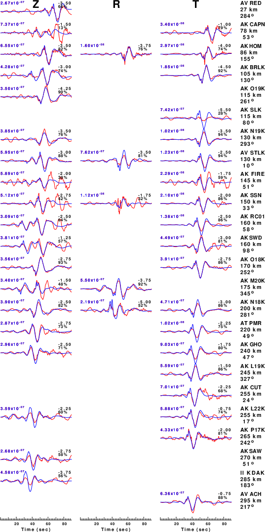
The comparison of the observed and predicted waveforms is given in the next figure. The red traces are the observed and the blue are the predicted.
Each observed-predicted component is plotted to the same scale and peak amplitudes are indicated by the numbers to the left of each trace. A pair of numbers is given in black at the right of each predicted traces. The upper number it the time shift required for maximum correlation between the observed and predicted traces. This time shift is required because the synthetics are not computed at exactly the same distance as the observed, the velocity model used in the predictions may not be perfect and the epicentral parameters may be be off.
A positive time shift indicates that the prediction is too fast and should be delayed to match the observed trace (shift to the right in this figure). A negative value indicates that the prediction is too slow. The lower number gives the percentage of variance reduction to characterize the individual goodness of fit (100% indicates a perfect fit).
The bandpass filter used in the processing and for the display was
cut o DIST/3.3 -50 o DIST/3.3 +40
rtr
taper w 0.1
hp c 0.03 n 3
lp c 0.07 n 3
br c 0.12 0.25 n 4 p 2
|
|
Figure 3. Waveform comparison for selected depth. Red: observed; Blue - predicted. The time shift with respect to the model prediction is indicated. The percent of fit is also indicated. The time scale is relative to the first trace sample.
|
|
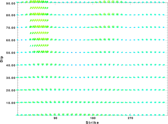
|
Focal mechanism sensitivity at the preferred depth. The red color indicates a very good fit to the waveforms.
Each solution is plotted as a vector at a given value of strike and dip with the angle of the vector representing the rake angle, measured, with respect to the upward vertical (N) in the figure.
|
Velocity Model
The WUS.model used for the waveform synthetic seismograms and for the surface wave eigenfunctions and dispersion is as follows
(The format is in the model96 format of Computer Programs in Seismology).
MODEL.01
Model after     8 iterations
ISOTROPIC
KGS
FLAT EARTH
1-D
CONSTANT VELOCITY
LINE08
LINE09
LINE10
LINE11
      H(KM)   VP(KM/S)   VS(KM/S) RHO(GM/CC)         QP         QS       ETAP       ETAS      FREFP      FREFS
     1.9000     3.4065     2.0089     2.2150  0.302E-02  0.679E-02   0.00       0.00       1.00       1.00
     6.1000     5.5445     3.2953     2.6089  0.349E-02  0.784E-02   0.00       0.00       1.00       1.00
    13.0000     6.2708     3.7396     2.7812  0.212E-02  0.476E-02   0.00       0.00       1.00       1.00
    19.0000     6.4075     3.7680     2.8223  0.111E-02  0.249E-02   0.00       0.00       1.00       1.00
     0.0000     7.9000     4.6200     3.2760  0.164E-10  0.370E-10   0.00       0.00       1.00       1.00
Last Changed Fri Dec 20 06:28:22 CST 2024