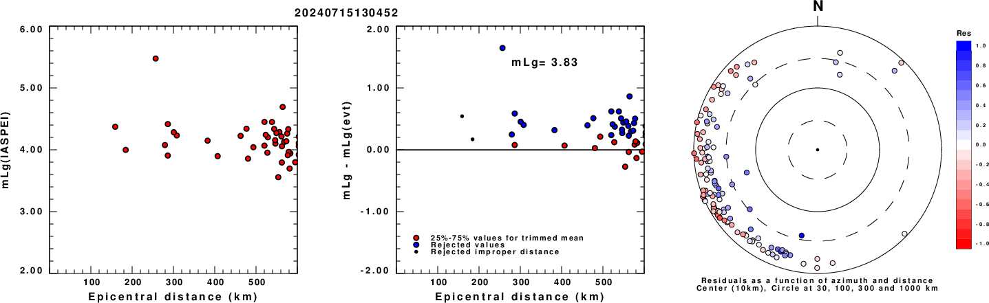
Left: mLg computed using the IASPEI formula. Center: mLg residuals versus epicentral distance ; the values used for the trimmed mean magnitude estimate are indicated. Right: residuals as a function of distance and azimuth.
The ANSS event ID is us7000mzc0 and the event page is at https://earthquake.usgs.gov/earthquakes/eventpage/us7000mzc0/executive.
2024/07/15 13:04:52 65.875 -135.086 13.0 4.1 Yukon, Canada
 USGS/SLU Moment Tensor Solution
 ENS  2024/07/15 13:04:52:0  65.88 -135.09  13.0 4.1  Yukon, Canada

 Stations used:
   AK.C27K AK.DOT AK.E25K AK.E27K AK.G24K AK.GREN AK.GRES
   AK.HDA AK.I27K AK.PAX AK.POKR AK.PPD AK.PS08 AK.RIDG
   CN.BRWY CN.CROWY CN.DAWY CN.HYT CN.INK CN.WHY CN.YUK4
   CN.YUK5 CN.YUK8 IU.COLA NY.MAYO PQ.OGILY PQ.TSIIG US.EGAK

 Filtering commands used:
   cut o DIST/3.3 -30 o DIST/3.3 +60
   rtr
   taper w 0.1
   hp c 0.03 n 3
   lp c 0.08 n 3

 Best Fitting Double Couple
  Mo = 9.55e+21 dyne-cm
  Mw = 3.92
  Z  = 26 km
  Plane   Strike  Dip  Rake
   NP1       40    65   -35
   NP2      146    59   -150
  Principal Axes:
   Axis    Value   Plunge  Azimuth
    T   9.55e+21      4      94
    N   0.00e+00     48     189
    P  -9.55e+21     42       1

 Moment Tensor: (dyne-cm)
    Component   Value
       Mxx    -5.25e+21
       Mxy    -8.35e+20
       Mxz    -4.80e+21
       Myy     9.44e+21
       Myz     5.72e+20
       Mzz    -4.20e+21


                     --------------
                 ----------------------
              ##-------------------------#
             ###-----------   -----------##
           #####----------- P -----------####
          ######-----------   -----------#####
         #######------------------------#######
        #########----------------------#########
        #########----------------------#########
       ###########--------------------###########
       ###########-------------------##########
       ############----------------############ T
       #############--------------#############
        ##############----------################
        ###############--------#################
         ###############-----##################
          ################-###################
           #############----#################
             ########----------############
              ##------------------########
                 ----------------------
                     --------------


 Global CMT Convention Moment Tensor:
      R          T          P
 -4.20e+21  -4.80e+21  -5.72e+20
 -4.80e+21  -5.25e+21   8.35e+20
 -5.72e+20   8.35e+20   9.44e+21


Details of the solution is found at

http://www.eas.slu.edu/eqc/eqc_mt/MECH.NA/20240715130452/index.html
|
      STK = 40
      DIP = 65
     RAKE = -35
       MW = 3.92
       HS = 26.0
The NDK file is 20240715130452.ndk The waveform inversion is preferred.
Given the availability of digital waveforms for determination of the moment tensor, this section documents the added processing leading to mLg, if appropriate to the region, and ML by application of the respective IASPEI formulae. As a research study, the linear distance term of the IASPEI formula for ML is adjusted to remove a linear distance trend in residuals to give a regionally defined ML. The defined ML uses horizontal component recordings, but the same procedure is applied to the vertical components since there may be some interest in vertical component ground motions. Residual plots versus distance may indicate interesting features of ground motion scaling in some distance ranges. A residual plot of the regionalized magnitude is given as a function of distance and azimuth, since data sets may transcend different wave propagation provinces.
Left: mLg computed using the IASPEI formula. Center: mLg residuals versus epicentral distance ; the values used for the trimmed mean magnitude estimate are indicated.
Right: residuals as a function of distance and azimuth.
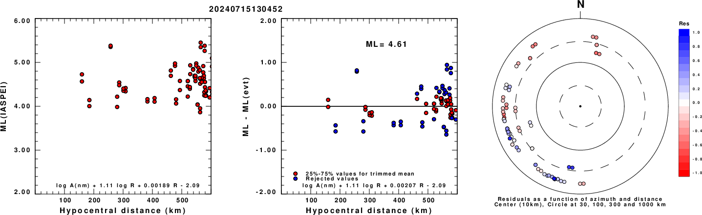
Left: ML computed using the IASPEI formula for Horizontal components. Center: ML residuals computed using a modified IASPEI formula that accounts for path specific attenuation; the values used for the trimmed mean are indicated. The ML relation used for each figure is given at the bottom of each plot.
Right: Residuals from new relation as a function of distance and azimuth.
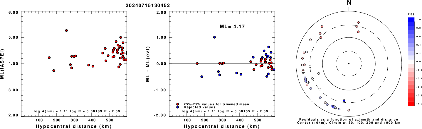
Left: ML computed using the IASPEI formula for Vertical components (research). Center: ML residuals computed using a modified IASPEI formula that accounts for path specific attenuation; the values used for the trimmed mean are indicated. The ML relation used for each figure is given at the bottom of each plot.
Right: Residuals from new relation as a function of distance and azimuth.
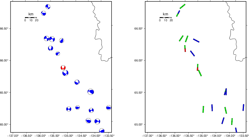 |
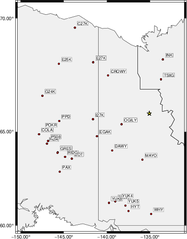
The focal mechanism was determined using broadband seismic waveforms. The location of the event (star) and the stations used for (red) the waveform inversion are shown in the next figure.
|
|
|
The program wvfgrd96 was used with good traces observed at short distance to determine the focal mechanism, depth and seismic moment. This technique requires a high quality signal and well determined velocity model for the Green's functions. To the extent that these are the quality data, this type of mechanism should be preferred over the radiation pattern technique which requires the separate step of defining the pressure and tension quadrants and the correct strike.
The observed and predicted traces are filtered using the following gsac commands:
cut o DIST/3.3 -30 o DIST/3.3 +60
rtr
taper w 0.1
hp c 0.03 n 3
lp c 0.08 n 3
The results of this grid search are as follow:
           DEPTH  STK   DIP  RAKE   MW    FIT
WVFGRD96    1.0   260    60    70   3.63 0.3029
WVFGRD96    2.0   275    50    85   3.71 0.3550
WVFGRD96    3.0   270    50    80   3.76 0.3399
WVFGRD96    4.0    45    70   -25   3.65 0.2930
WVFGRD96    5.0    45    70   -30   3.66 0.2932
WVFGRD96    6.0    45    70   -30   3.67 0.2933
WVFGRD96    7.0    45    60   -25   3.67 0.3011
WVFGRD96    8.0    45    60   -25   3.68 0.3128
WVFGRD96    9.0    45    60   -25   3.69 0.3274
WVFGRD96   10.0    40    55   -30   3.72 0.3390
WVFGRD96   11.0    40    60   -35   3.74 0.3541
WVFGRD96   12.0    40    60   -35   3.75 0.3696
WVFGRD96   13.0    40    60   -35   3.77 0.3840
WVFGRD96   14.0    40    60   -35   3.78 0.3968
WVFGRD96   15.0    40    60   -35   3.79 0.4088
WVFGRD96   16.0    40    60   -35   3.80 0.4197
WVFGRD96   17.0    40    60   -35   3.81 0.4299
WVFGRD96   18.0    40    60   -35   3.82 0.4394
WVFGRD96   19.0    40    60   -35   3.83 0.4485
WVFGRD96   20.0    40    60   -35   3.86 0.4523
WVFGRD96   21.0    40    60   -35   3.87 0.4589
WVFGRD96   22.0    40    65   -35   3.89 0.4646
WVFGRD96   23.0    40    65   -35   3.89 0.4688
WVFGRD96   24.0    40    65   -35   3.90 0.4715
WVFGRD96   25.0    40    65   -35   3.91 0.4727
WVFGRD96   26.0    40    65   -35   3.92 0.4729
WVFGRD96   27.0    40    65   -35   3.93 0.4716
WVFGRD96   28.0    40    65   -35   3.94 0.4696
WVFGRD96   29.0    40    65   -35   3.95 0.4667
WVFGRD96   30.0    40    65   -35   3.95 0.4630
WVFGRD96   31.0    40    65   -35   3.96 0.4587
WVFGRD96   32.0    50    75   -50   3.98 0.4551
WVFGRD96   33.0    50    75   -50   3.99 0.4506
WVFGRD96   34.0    50    75   -50   4.00 0.4461
WVFGRD96   35.0    50    75   -50   4.00 0.4418
WVFGRD96   36.0    45    75   -45   4.01 0.4372
WVFGRD96   37.0    45    70   -40   4.02 0.4343
WVFGRD96   38.0    45    70   -40   4.04 0.4318
WVFGRD96   39.0    40    65   -35   4.05 0.4296
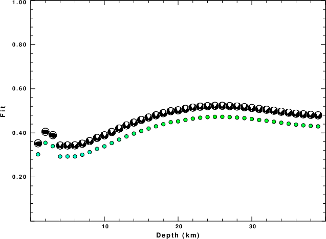
The best solution is
WVFGRD96 26.0 40 65 -35 3.92 0.4729
The mechanism corresponding to the best fit is
|
|
|
The best fit as a function of depth is given in the following figure:
|
|
|
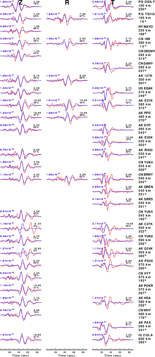
The comparison of the observed and predicted waveforms is given in the next figure. The red traces are the observed and the blue are the predicted. Each observed-predicted component is plotted to the same scale and peak amplitudes are indicated by the numbers to the left of each trace. A pair of numbers is given in black at the right of each predicted traces. The upper number it the time shift required for maximum correlation between the observed and predicted traces. This time shift is required because the synthetics are not computed at exactly the same distance as the observed, the velocity model used in the predictions may not be perfect and the epicentral parameters may be be off. A positive time shift indicates that the prediction is too fast and should be delayed to match the observed trace (shift to the right in this figure). A negative value indicates that the prediction is too slow. The lower number gives the percentage of variance reduction to characterize the individual goodness of fit (100% indicates a perfect fit).
The bandpass filter used in the processing and for the display was
cut o DIST/3.3 -30 o DIST/3.3 +60
rtr
taper w 0.1
hp c 0.03 n 3
lp c 0.08 n 3
|
| Figure 3. Waveform comparison for selected depth. Red: observed; Blue - predicted. The time shift with respect to the model prediction is indicated. The percent of fit is also indicated. The time scale is relative to the first trace sample. |
|
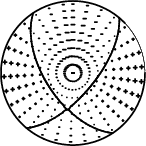
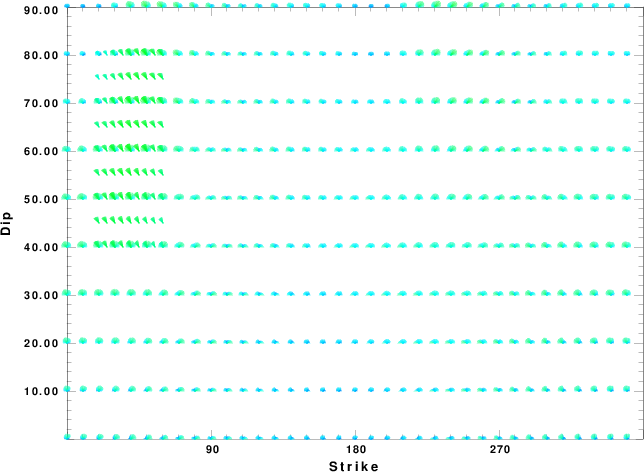
| Focal mechanism sensitivity at the preferred depth. The red color indicates a very good fit to the waveforms. Each solution is plotted as a vector at a given value of strike and dip with the angle of the vector representing the rake angle, measured, with respect to the upward vertical (N) in the figure. |
A check on the assumed source location is possible by looking at the time shifts between the observed and predicted traces. The time shifts for waveform matching arise for several reasons:
Time_shift = A + B cos Azimuth + C Sin Azimuth
The time shifts for this inversion lead to the next figure:
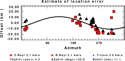
The derived shift in origin time and epicentral coordinates are given at the bottom of the figure.
The CUS.model used for the waveform synthetic seismograms and for the surface wave eigenfunctions and dispersion is as follows (The format is in the model96 format of Computer Programs in Seismology).
MODEL.01
CUS Model with Q from simple gamma values
ISOTROPIC
KGS
FLAT EARTH
1-D
CONSTANT VELOCITY
LINE08
LINE09
LINE10
LINE11
  H(KM) VP(KM/S) VS(KM/S) RHO(GM/CC)   QP   QS  ETAP  ETAS  FREFP  FREFS
  1.0000  5.0000  2.8900  2.5000 0.172E-02 0.387E-02 0.00  0.00  1.00  1.00
  9.0000  6.1000  3.5200  2.7300 0.160E-02 0.363E-02 0.00  0.00  1.00  1.00
 10.0000  6.4000  3.7000  2.8200 0.149E-02 0.336E-02 0.00  0.00  1.00  1.00
 20.0000  6.7000  3.8700  2.9020 0.000E-04 0.000E-04 0.00  0.00  1.00  1.00
  0.0000  8.1500  4.7000  3.3640 0.194E-02 0.431E-02 0.00  0.00  1.00  1.00