Location
Location ANSS
The ANSS event ID is us7000mx7h and the event page is at
https://earthquake.usgs.gov/earthquakes/eventpage/us7000mx7h/executive.
2024/07/05 10:46:38 47.289 -113.214 10.0 3.9 Montana
Focal Mechanism
 USGS/SLU Moment Tensor Solution
 ENS  2024/07/05 10:46:38:0  47.29 -113.21  10.0 3.9 Montana

 Stations used:
   IW.DLMT IW.PLID MB.ECMT MB.FCMT MB.GBMT MB.HRY MB.JTMT
   MB.LDM MB.LRM MB.SRMT US.BMO US.BOZ US.EGMT US.HLID US.MSO
   US.NEW US.RLMT UW.AGNW UW.BRAN UW.DAVN UW.LBRT UW.LMONT
   UW.LNO UW.TUCA UW.WOLL WW.BILL WW.IRMR WY.YFT WY.YHB WY.YHL
   WY.YMR WY.YNE WY.YNR

 Filtering commands used:
   cut o DIST/3.3 -40 o DIST/3.3 +50
   rtr
   taper w 0.1
   hp c 0.03 n 3
   lp c 0.08 n 3

 Best Fitting Double Couple
  Mo = 6.76e+21 dyne-cm
  Mw = 3.82
  Z  = 24 km
  Plane   Strike  Dip  Rake
   NP1       40    75   -25
   NP2      137    66   -164
  Principal Axes:
   Axis    Value   Plunge  Azimuth
    T   6.76e+21      6      90
    N   0.00e+00     61     191
    P  -6.76e+21     28     357

 Moment Tensor: (dyne-cm)
    Component   Value
       Mxx    -5.24e+21
       Mxy     3.24e+20
       Mxz    -2.81e+21
       Myy     6.67e+21
       Myz     8.76e+20
       Mzz    -1.43e+21


                     --------------
                 ---------   ----------
              ------------ P ------------#
             #------------   ------------##
           ###--------------------------#####
          #####------------------------#######
         ######-----------------------#########
        ########---------------------###########
        #########-------------------############
       ###########-----------------###########
       ############---------------############ T
       ##############-----------##############
       ###############---------##################
        ################-----###################
        ##################-#####################
         ################---###################
          #############-------################
           ##########------------############
             ######------------------######
              #---------------------------
                 ----------------------
                     --------------


 Global CMT Convention Moment Tensor:
      R          T          P
 -1.43e+21  -2.81e+21  -8.76e+20
 -2.81e+21  -5.24e+21  -3.24e+20
 -8.76e+20  -3.24e+20   6.67e+21


Details of the solution is found at

http://www.eas.slu.edu/eqc/eqc_mt/MECH.NA/20240705104638/index.html
|
Preferred Solution
The preferred solution from an analysis of the surface-wave spectral amplitude radiation pattern, waveform inversion or first motion observations is
      STK = 40
      DIP = 75
     RAKE = -25
       MW = 3.82
       HS = 24.0
The NDK file is 20240705104638.ndk
The waveform inversion is preferred.
Magnitudes
Given the availability of digital waveforms for determination of the moment tensor, this section documents the added processing leading to mLg, if appropriate to the region, and ML by application of the respective IASPEI formulae. As a research study, the linear distance term of the IASPEI formula
for ML is adjusted to remove a linear distance trend in residuals to give a regionally defined ML. The defined ML uses horizontal component recordings, but the same procedure is applied to the vertical components since there may be some interest in vertical component ground motions. Residual plots versus distance may indicate interesting features of ground motion scaling in some distance ranges. A residual plot of the regionalized magnitude is given as a function of distance and azimuth, since data sets may transcend different wave propagation provinces.
ML Magnitude
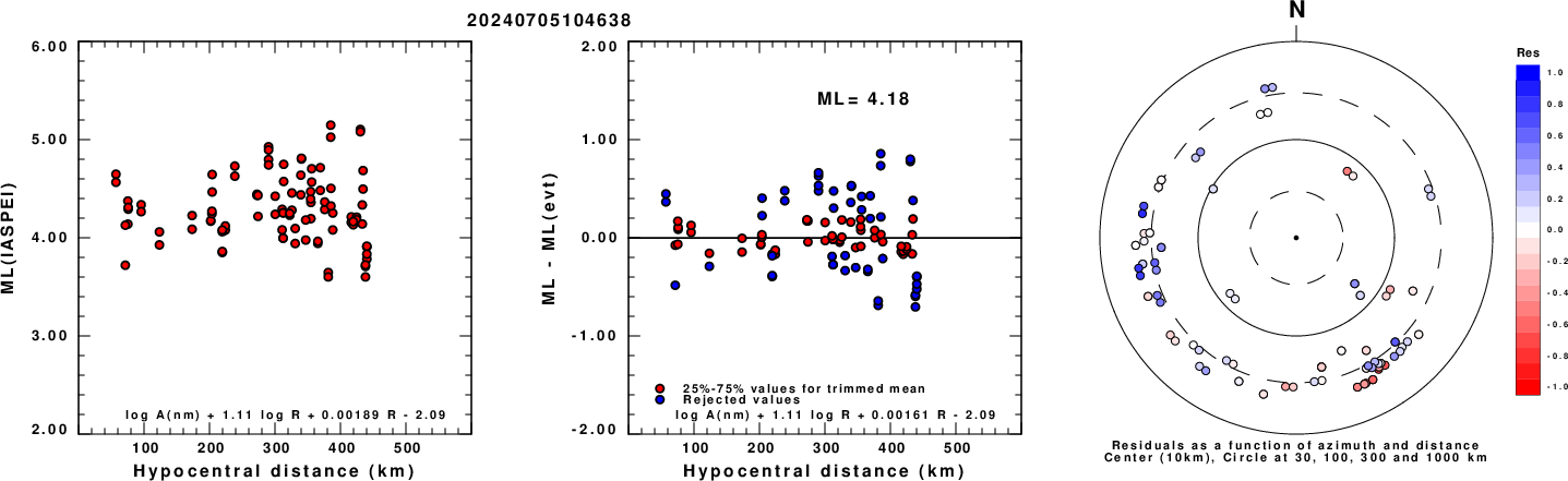
Left: ML computed using the IASPEI formula for Horizontal components. Center: ML residuals computed using a modified IASPEI formula that accounts for path specific attenuation; the values used for the trimmed mean are indicated. The ML relation used for each figure is given at the bottom of each plot.
Right: Residuals from new relation as a function of distance and azimuth.
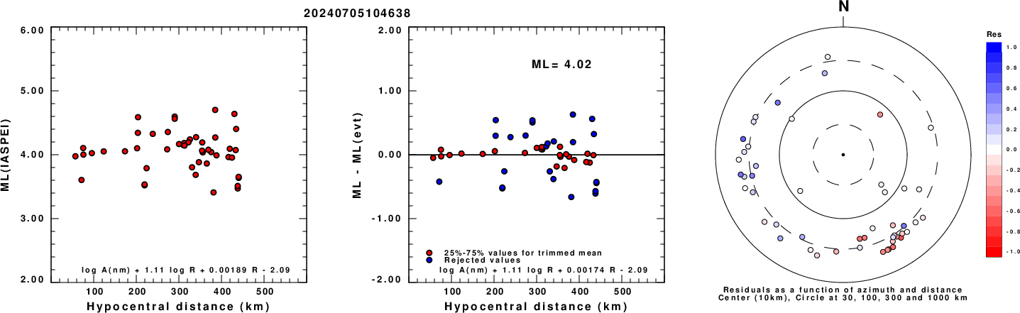
Left: ML computed using the IASPEI formula for Vertical components (research). Center: ML residuals computed using a modified IASPEI formula that accounts for path specific attenuation; the values used for the trimmed mean are indicated. The ML relation used for each figure is given at the bottom of each plot.
Right: Residuals from new relation as a function of distance and azimuth.
Context
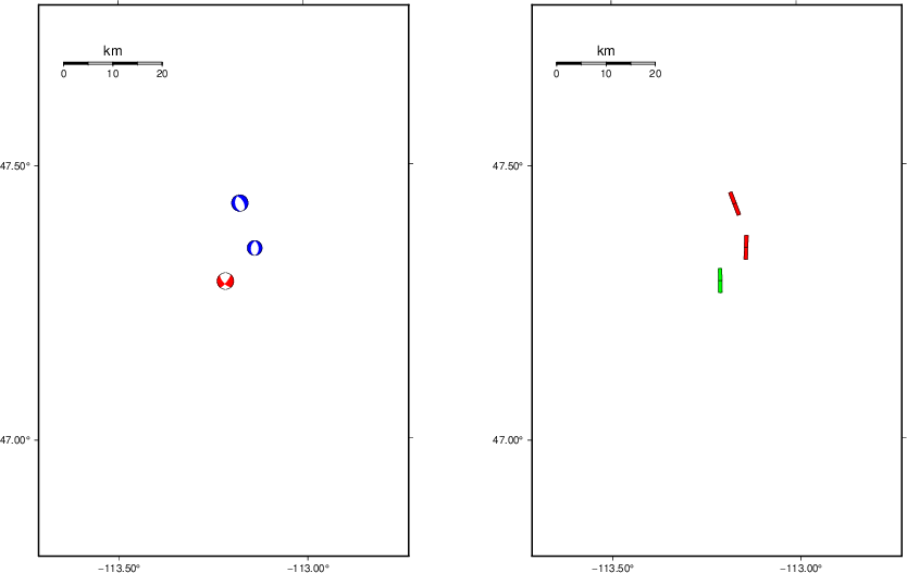
The left panel of the next figure presents the focal mechanism for this earthquake (red) in the context of other nearby events (blue) in the SLU Moment Tensor Catalog. The right panel shows the inferred direction of maximum compressive stress and the type of faulting (green is strike-slip, red is normal, blue is thrust; oblique is shown by a combination of colors). Thus context plot is useful for assessing the appropriateness of the moment tensor of this event.
Waveform Inversion using wvfgrd96
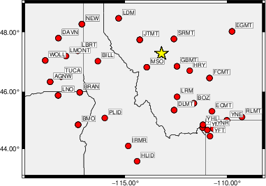
The focal mechanism was determined using broadband seismic waveforms. The location of the event (star) and the
stations used for (red) the waveform inversion are shown in the next figure.
|
|
Location of broadband stations used for waveform inversion
|
The program wvfgrd96 was used with good traces observed at short distance to determine the focal mechanism, depth and seismic moment. This technique requires a high quality signal and well determined velocity model for the Green's functions. To the extent that these are the quality data, this type of mechanism should be preferred over the radiation pattern technique which requires the separate step of defining the pressure and tension quadrants and the correct strike.
The observed and predicted traces are filtered using the following gsac commands:
cut o DIST/3.3 -40 o DIST/3.3 +50
rtr
taper w 0.1
hp c 0.03 n 3
lp c 0.08 n 3
The results of this grid search are as follow:
           DEPTH  STK   DIP  RAKE   MW    FIT
WVFGRD96    1.0   165    50    65   3.31 0.2757
WVFGRD96    2.0   160    50    60   3.44 0.3848
WVFGRD96    3.0   230    75   -15   3.40 0.4159
WVFGRD96    4.0   225    85    25   3.44 0.4522
WVFGRD96    5.0   225    80    25   3.48 0.4950
WVFGRD96    6.0   225    80    25   3.51 0.5367
WVFGRD96    7.0   225    80    25   3.55 0.5768
WVFGRD96    8.0   225    80    30   3.60 0.6146
WVFGRD96    9.0   225    80    30   3.62 0.6431
WVFGRD96   10.0   225    80    25   3.64 0.6678
WVFGRD96   11.0   225    80    25   3.66 0.6892
WVFGRD96   12.0   225    80    25   3.68 0.7070
WVFGRD96   13.0   225    80    25   3.69 0.7219
WVFGRD96   14.0    40    80   -25   3.71 0.7338
WVFGRD96   15.0    40    80   -25   3.72 0.7470
WVFGRD96   16.0    40    75   -25   3.74 0.7580
WVFGRD96   17.0    40    75   -25   3.75 0.7688
WVFGRD96   18.0    40    75   -25   3.76 0.7777
WVFGRD96   19.0    40    75   -25   3.77 0.7851
WVFGRD96   20.0    40    75   -25   3.79 0.7908
WVFGRD96   21.0    40    75   -25   3.80 0.7956
WVFGRD96   22.0    40    75   -25   3.81 0.7998
WVFGRD96   23.0    40    75   -25   3.81 0.8024
WVFGRD96   24.0    40    75   -25   3.82 0.8036
WVFGRD96   25.0    40    75   -25   3.83 0.8034
WVFGRD96   26.0    40    75   -25   3.84 0.8015
WVFGRD96   27.0    40    75   -25   3.84 0.7979
WVFGRD96   28.0    40    75   -25   3.85 0.7931
WVFGRD96   29.0    40    75   -25   3.86 0.7864
WVFGRD96   30.0    40    75   -25   3.86 0.7775
WVFGRD96   31.0    40    75   -25   3.87 0.7672
WVFGRD96   32.0    40    75   -25   3.87 0.7554
WVFGRD96   33.0    40    75   -25   3.88 0.7419
WVFGRD96   34.0    40    75   -25   3.88 0.7282
WVFGRD96   35.0    40    75   -25   3.89 0.7134
WVFGRD96   36.0    40    75   -25   3.89 0.6997
WVFGRD96   37.0    40    75   -20   3.90 0.6874
WVFGRD96   38.0    40    75   -20   3.91 0.6773
WVFGRD96   39.0    40    75   -20   3.92 0.6703
WVFGRD96   40.0    35    65   -30   3.97 0.6687
WVFGRD96   41.0    35    65   -30   3.98 0.6658
WVFGRD96   42.0    35    65   -30   3.99 0.6627
WVFGRD96   43.0    40    70   -25   3.99 0.6598
WVFGRD96   44.0    40    70   -25   3.99 0.6570
WVFGRD96   45.0    40    65   -25   4.01 0.6537
WVFGRD96   46.0    40    70   -25   4.01 0.6497
WVFGRD96   47.0    40    70   -25   4.01 0.6455
WVFGRD96   48.0    40    70   -20   4.01 0.6409
WVFGRD96   49.0    40    70   -20   4.02 0.6367
WVFGRD96   50.0    40    70   -20   4.03 0.6336
WVFGRD96   51.0    40    75   -20   4.03 0.6309
WVFGRD96   52.0    40    75   -20   4.03 0.6267
WVFGRD96   53.0    40    75   -20   4.04 0.6229
WVFGRD96   54.0    40    75   -20   4.04 0.6210
WVFGRD96   55.0    40    75   -20   4.04 0.6175
WVFGRD96   56.0    40    75   -20   4.05 0.6142
WVFGRD96   57.0    40    75   -20   4.05 0.6132
WVFGRD96   58.0    40    75   -20   4.06 0.6095
WVFGRD96   59.0    40    80   -15   4.06 0.6076
The best solution is
WVFGRD96 24.0 40 75 -25 3.82 0.8036
The mechanism corresponding to the best fit is
|
|
Figure 1. Waveform inversion focal mechanism
|
The best fit as a function of depth is given in the following figure:
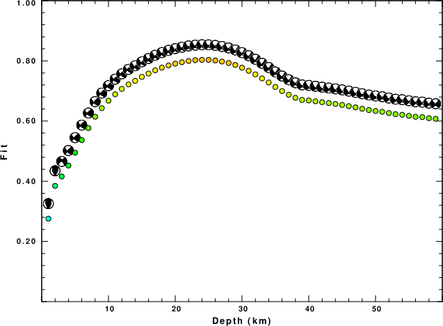
|
|
Figure 2. Depth sensitivity for waveform mechanism
|
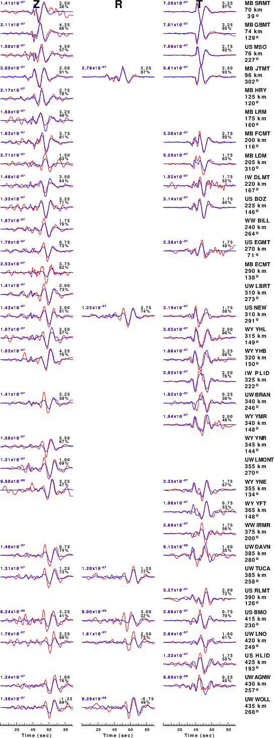
The comparison of the observed and predicted waveforms is given in the next figure. The red traces are the observed and the blue are the predicted.
Each observed-predicted component is plotted to the same scale and peak amplitudes are indicated by the numbers to the left of each trace. A pair of numbers is given in black at the right of each predicted traces. The upper number it the time shift required for maximum correlation between the observed and predicted traces. This time shift is required because the synthetics are not computed at exactly the same distance as the observed, the velocity model used in the predictions may not be perfect and the epicentral parameters may be be off.
A positive time shift indicates that the prediction is too fast and should be delayed to match the observed trace (shift to the right in this figure). A negative value indicates that the prediction is too slow. The lower number gives the percentage of variance reduction to characterize the individual goodness of fit (100% indicates a perfect fit).
The bandpass filter used in the processing and for the display was
cut o DIST/3.3 -40 o DIST/3.3 +50
rtr
taper w 0.1
hp c 0.03 n 3
lp c 0.08 n 3
|
|
Figure 3. Waveform comparison for selected depth. Red: observed; Blue - predicted. The time shift with respect to the model prediction is indicated. The percent of fit is also indicated. The time scale is relative to the first trace sample.
|
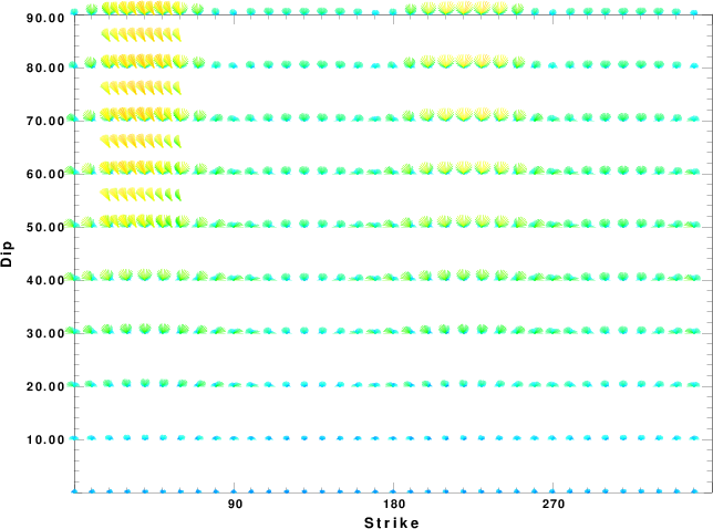
|
|
Focal mechanism sensitivity at the preferred depth. The red color indicates a very good fit to the waveforms.
Each solution is plotted as a vector at a given value of strike and dip with the angle of the vector representing the rake angle, measured, with respect to the upward vertical (N) in the figure.
|
A check on the assumed source location is possible by looking at the time shifts between the observed and predicted traces. The time shifts for waveform matching arise for several reasons:
- The origin time and epicentral distance are incorrect
- The velocity model used for the inversion is incorrect
- The velocity model used to define the P-arrival time is not the
same as the velocity model used for the waveform inversion
(assuming that the initial trace alignment is based on the
P arrival time)
Assuming only a mislocation, the time shifts are fit to a functional form:
Time_shift = A + B cos Azimuth + C Sin Azimuth
The time shifts for this inversion lead to the next figure:
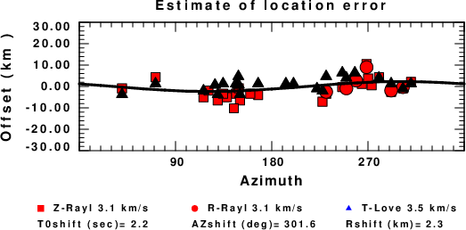
The derived shift in origin time and epicentral coordinates are given at the bottom of the figure.
Velocity Model
The WUS.model used for the waveform synthetic seismograms and for the surface wave eigenfunctions and dispersion is as follows
(The format is in the model96 format of Computer Programs in Seismology).
MODEL.01
Model after     8 iterations
ISOTROPIC
KGS
FLAT EARTH
1-D
CONSTANT VELOCITY
LINE08
LINE09
LINE10
LINE11
      H(KM)   VP(KM/S)   VS(KM/S) RHO(GM/CC)         QP         QS       ETAP       ETAS      FREFP      FREFS
     1.9000     3.4065     2.0089     2.2150  0.302E-02  0.679E-02   0.00       0.00       1.00       1.00
     6.1000     5.5445     3.2953     2.6089  0.349E-02  0.784E-02   0.00       0.00       1.00       1.00
    13.0000     6.2708     3.7396     2.7812  0.212E-02  0.476E-02   0.00       0.00       1.00       1.00
    19.0000     6.4075     3.7680     2.8223  0.111E-02  0.249E-02   0.00       0.00       1.00       1.00
     0.0000     7.9000     4.6200     3.2760  0.164E-10  0.370E-10   0.00       0.00       1.00       1.00
Last Changed Fri Jul 5 07:01:15 CDT 2024