Location
Location ANSS
The ANSS event ID is us7000mpmr and the event page is at
https://earthquake.usgs.gov/earthquakes/eventpage/us7000mpmr/executive.
2024/06/02 14:02:42 65.791 -135.007 15.6 4.9 Yukon, Canada
Focal Mechanism
 USGS/SLU Moment Tensor Solution
 ENS  2024/06/02 14:02:42:0  65.79 -135.01  15.6 4.9  Yukon, Canada

 Stations used:
   AK.BAL AK.BARN AK.C27K AK.DOT AK.E25K AK.E27K AK.GREN
   AK.GRES AK.HDA AK.I27K AK.K24K AK.LOGN AK.MCAR AK.POKR
   AK.PPD AK.PS08 AK.PS09 AK.PS10 AK.RIDG AK.SCRK AK.VRDI
   AK.WRH AT.MENT CN.BRWY CN.BVCY CN.CROWY CN.DAWY CN.HYT
   CN.INK CN.WHY CN.YUK3 CN.YUK4 CN.YUK5 CN.YUK6 CN.YUK7
   CN.YUK8 EO.KLRS IM.IL31 IU.COLA NY.MAYO NY.MMPY PQ.OGILY
   PQ.TSIIG PQ.TUKN US.EGAK

 Filtering commands used:
   cut o DIST/3.3 -40 o DIST/3.3 +50
   rtr
   taper w 0.1
   hp c 0.03 n 3
   lp c 0.07 n 3

 Best Fitting Double Couple
  Mo = 2.21e+23 dyne-cm
  Mw = 4.83
  Z  = 26 km
  Plane   Strike  Dip  Rake
   NP1      122    74   -143
   NP2       20    55   -20
  Principal Axes:
   Axis    Value   Plunge  Azimuth
    T   2.21e+23     12     247
    N   0.00e+00     50     142
    P  -2.21e+23     37     346

 Moment Tensor: (dyne-cm)
    Component   Value
       Mxx    -1.01e+23
       Mxy     1.08e+23
       Mxz    -1.21e+23
       Myy     1.72e+23
       Myz    -1.65e+22
       Mzz    -7.11e+22


                     --------------
                 -------------------###
              -----------------------#####
             ----------   ------------#####
           ------------ P ------------#######
          #------------   ------------########
         ###--------------------------#########
        ######------------------------##########
        #######-----------------------##########
       ##########---------------------###########
       ############------------------############
       ###############---------------############
       ##################-----------#############
        #   ################--------############
        # T ###################----#############
            ######################-############
          #######################--------#####
           ####################--------------
             #################-------------
              ##############--------------
                 ########--------------
                     --------------


 Global CMT Convention Moment Tensor:
      R          T          P
 -7.11e+22  -1.21e+23   1.65e+22
 -1.21e+23  -1.01e+23  -1.08e+23
  1.65e+22  -1.08e+23   1.72e+23


Details of the solution is found at

http://www.eas.slu.edu/eqc/eqc_mt/MECH.NA/20240602140242/index.html
|
Preferred Solution
The preferred solution from an analysis of the surface-wave spectral amplitude radiation pattern, waveform inversion or first motion observations is
      STK = 20
      DIP = 55
     RAKE = -20
       MW = 4.83
       HS = 26.0
The NDK file is 20240602140242.ndk
The waveform inversion is preferred.
Moment Tensor Comparison
The following compares this source inversion to those provided by others. The purpose is to look for major differences and also to note slight differences that might be inherent to the processing procedure. For completeness the USGS/SLU solution is repeated from above.
| SLU |
USGSW |
 USGS/SLU Moment Tensor Solution
 ENS  2024/06/02 14:02:42:0  65.79 -135.01  15.6 4.9  Yukon, Canada

 Stations used:
   AK.BAL AK.BARN AK.C27K AK.DOT AK.E25K AK.E27K AK.GREN
   AK.GRES AK.HDA AK.I27K AK.K24K AK.LOGN AK.MCAR AK.POKR
   AK.PPD AK.PS08 AK.PS09 AK.PS10 AK.RIDG AK.SCRK AK.VRDI
   AK.WRH AT.MENT CN.BRWY CN.BVCY CN.CROWY CN.DAWY CN.HYT
   CN.INK CN.WHY CN.YUK3 CN.YUK4 CN.YUK5 CN.YUK6 CN.YUK7
   CN.YUK8 EO.KLRS IM.IL31 IU.COLA NY.MAYO NY.MMPY PQ.OGILY
   PQ.TSIIG PQ.TUKN US.EGAK

 Filtering commands used:
   cut o DIST/3.3 -40 o DIST/3.3 +50
   rtr
   taper w 0.1
   hp c 0.03 n 3
   lp c 0.07 n 3

 Best Fitting Double Couple
  Mo = 2.21e+23 dyne-cm
  Mw = 4.83
  Z  = 26 km
  Plane   Strike  Dip  Rake
   NP1      122    74   -143
   NP2       20    55   -20
  Principal Axes:
   Axis    Value   Plunge  Azimuth
    T   2.21e+23     12     247
    N   0.00e+00     50     142
    P  -2.21e+23     37     346

 Moment Tensor: (dyne-cm)
    Component   Value
       Mxx    -1.01e+23
       Mxy     1.08e+23
       Mxz    -1.21e+23
       Myy     1.72e+23
       Myz    -1.65e+22
       Mzz    -7.11e+22


                     --------------
                 -------------------###
              -----------------------#####
             ----------   ------------#####
           ------------ P ------------#######
          #------------   ------------########
         ###--------------------------#########
        ######------------------------##########
        #######-----------------------##########
       ##########---------------------###########
       ############------------------############
       ###############---------------############
       ##################-----------#############
        #   ################--------############
        # T ###################----#############
            ######################-############
          #######################--------#####
           ####################--------------
             #################-------------
              ##############--------------
                 ########--------------
                     --------------


 Global CMT Convention Moment Tensor:
      R          T          P
 -7.11e+22  -1.21e+23   1.65e+22
 -1.21e+23  -1.01e+23  -1.08e+23
  1.65e+22  -1.08e+23   1.72e+23


Details of the solution is found at

http://www.eas.slu.edu/eqc/eqc_mt/MECH.NA/20240602140242/index.html
|
W-phase Moment Tensor (Mww)
Moment
2.391e+16 N-m
Magnitude
4.85 Mww
Depth
23.5 km
Percent DC
97%
Half Duration
0.50 s
Catalog
US
Data Source
US 2
Contributor
US 2
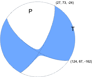
Nodal Planes
Plane Strike Dip Rake
NP1 27 73 -24
NP2 124 67 -162
Principal Axes
Axis Value Plunge Azimuth
T 2.371e+16 4 77
N 0.039e+16 61 174
P -2.410e+16 29 345
|
Magnitudes
Given the availability of digital waveforms for determination of the moment tensor, this section documents the added processing leading to mLg, if appropriate to the region, and ML by application of the respective IASPEI formulae. As a research study, the linear distance term of the IASPEI formula
for ML is adjusted to remove a linear distance trend in residuals to give a regionally defined ML. The defined ML uses horizontal component recordings, but the same procedure is applied to the vertical components since there may be some interest in vertical component ground motions. Residual plots versus distance may indicate interesting features of ground motion scaling in some distance ranges. A residual plot of the regionalized magnitude is given as a function of distance and azimuth, since data sets may transcend different wave propagation provinces.
mLg Magnitude
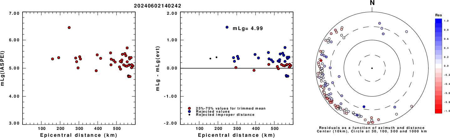
Left: mLg computed using the IASPEI formula. Center: mLg residuals versus epicentral distance ; the values used for the trimmed mean magnitude estimate are indicated.
Right: residuals as a function of distance and azimuth.
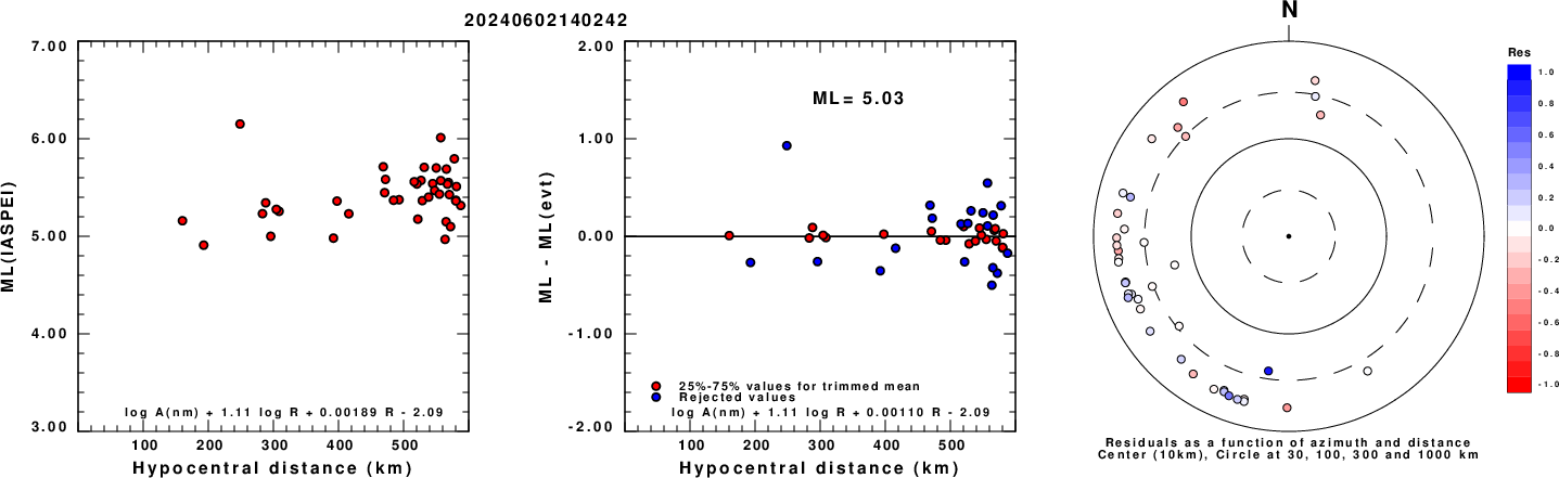
ML Magnitude
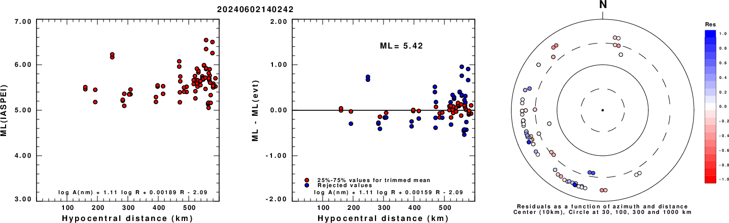
Left: ML computed using the IASPEI formula for Horizontal components. Center: ML residuals computed using a modified IASPEI formula that accounts for path specific attenuation; the values used for the trimmed mean are indicated. The ML relation used for each figure is given at the bottom of each plot.
Right: Residuals from new relation as a function of distance and azimuth.
Left: ML computed using the IASPEI formula for Vertical components (research). Center: ML residuals computed using a modified IASPEI formula that accounts for path specific attenuation; the values used for the trimmed mean are indicated. The ML relation used for each figure is given at the bottom of each plot.
Right: Residuals from new relation as a function of distance and azimuth.
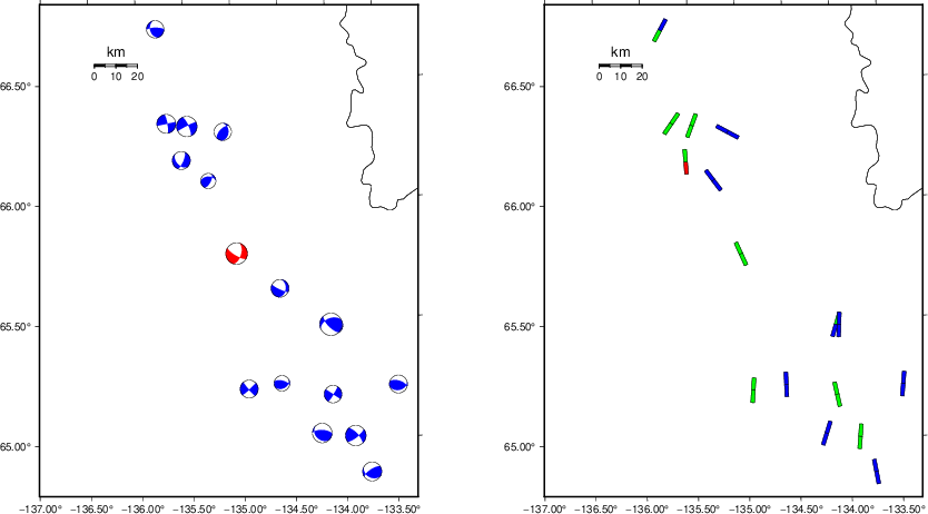
Context
The left panel of the next figure presents the focal mechanism for this earthquake (red) in the context of other nearby events (blue) in the SLU Moment Tensor Catalog. The right panel shows the inferred direction of maximum compressive stress and the type of faulting (green is strike-slip, red is normal, blue is thrust; oblique is shown by a combination of colors). Thus context plot is useful for assessing the appropriateness of the moment tensor of this event.
Waveform Inversion using wvfgrd96
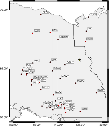
The focal mechanism was determined using broadband seismic waveforms. The location of the event (star) and the
stations used for (red) the waveform inversion are shown in the next figure.
|
|
Location of broadband stations used for waveform inversion
|
The program wvfgrd96 was used with good traces observed at short distance to determine the focal mechanism, depth and seismic moment. This technique requires a high quality signal and well determined velocity model for the Green's functions. To the extent that these are the quality data, this type of mechanism should be preferred over the radiation pattern technique which requires the separate step of defining the pressure and tension quadrants and the correct strike.
The observed and predicted traces are filtered using the following gsac commands:
cut o DIST/3.3 -40 o DIST/3.3 +50
rtr
taper w 0.1
hp c 0.03 n 3
lp c 0.07 n 3
The results of this grid search are as follow:
           DEPTH  STK   DIP  RAKE   MW    FIT
WVFGRD96    1.0    40    65    30   4.57 0.3388
WVFGRD96    2.0   250    45    90   4.66 0.3577
WVFGRD96    3.0    50    55    50   4.66 0.3472
WVFGRD96    4.0    35    55    10   4.60 0.3347
WVFGRD96    5.0    30    50     5   4.60 0.3429
WVFGRD96    6.0    30    50     5   4.61 0.3557
WVFGRD96    7.0    25    50     0   4.61 0.3705
WVFGRD96    8.0    25    50     0   4.61 0.3852
WVFGRD96    9.0    25    50    -5   4.62 0.3992
WVFGRD96   10.0    25    50    -5   4.65 0.4118
WVFGRD96   11.0    25    50    -5   4.66 0.4252
WVFGRD96   12.0    25    50   -20   4.68 0.4404
WVFGRD96   13.0    20    50   -25   4.69 0.4555
WVFGRD96   14.0    20    50   -25   4.70 0.4699
WVFGRD96   15.0    20    50   -25   4.71 0.4826
WVFGRD96   16.0    20    55   -25   4.72 0.4937
WVFGRD96   17.0    20    55   -25   4.73 0.5044
WVFGRD96   18.0    20    55   -25   4.74 0.5135
WVFGRD96   19.0    20    55   -25   4.75 0.5213
WVFGRD96   20.0    20    55   -25   4.78 0.5285
WVFGRD96   21.0    20    55   -25   4.79 0.5345
WVFGRD96   22.0    20    55   -25   4.80 0.5392
WVFGRD96   23.0    20    55   -25   4.80 0.5425
WVFGRD96   24.0    20    55   -20   4.81 0.5452
WVFGRD96   25.0    20    55   -20   4.82 0.5466
WVFGRD96   26.0    20    55   -20   4.83 0.5467
WVFGRD96   27.0    20    55   -20   4.84 0.5461
WVFGRD96   28.0    20    55   -20   4.85 0.5444
WVFGRD96   29.0    20    55   -20   4.86 0.5417
The best solution is
WVFGRD96 26.0 20 55 -20 4.83 0.5467
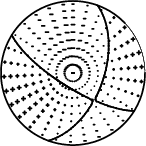
The mechanism corresponding to the best fit is
|
|
Figure 1. Waveform inversion focal mechanism
|
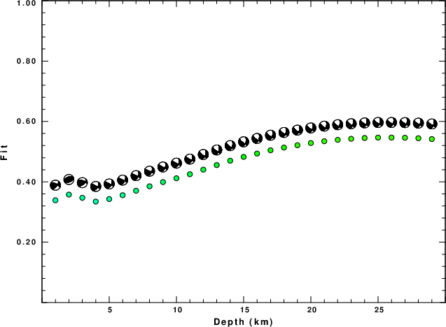
The best fit as a function of depth is given in the following figure:
|
|
Figure 2. Depth sensitivity for waveform mechanism
|
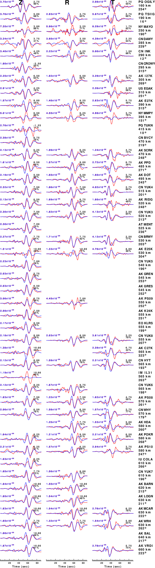
The comparison of the observed and predicted waveforms is given in the next figure. The red traces are the observed and the blue are the predicted.
Each observed-predicted component is plotted to the same scale and peak amplitudes are indicated by the numbers to the left of each trace. A pair of numbers is given in black at the right of each predicted traces. The upper number it the time shift required for maximum correlation between the observed and predicted traces. This time shift is required because the synthetics are not computed at exactly the same distance as the observed, the velocity model used in the predictions may not be perfect and the epicentral parameters may be be off.
A positive time shift indicates that the prediction is too fast and should be delayed to match the observed trace (shift to the right in this figure). A negative value indicates that the prediction is too slow. The lower number gives the percentage of variance reduction to characterize the individual goodness of fit (100% indicates a perfect fit).
The bandpass filter used in the processing and for the display was
cut o DIST/3.3 -40 o DIST/3.3 +50
rtr
taper w 0.1
hp c 0.03 n 3
lp c 0.07 n 3
|
|
Figure 3. Waveform comparison for selected depth. Red: observed; Blue - predicted. The time shift with respect to the model prediction is indicated. The percent of fit is also indicated. The time scale is relative to the first trace sample.
|
|
|
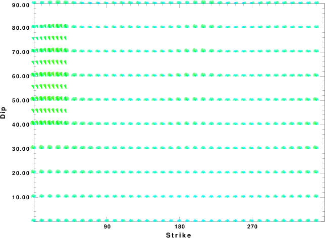
Focal mechanism sensitivity at the preferred depth. The red color indicates a very good fit to the waveforms.
Each solution is plotted as a vector at a given value of strike and dip with the angle of the vector representing the rake angle, measured, with respect to the upward vertical (N) in the figure.
|
A check on the assumed source location is possible by looking at the time shifts between the observed and predicted traces. The time shifts for waveform matching arise for several reasons:
- The origin time and epicentral distance are incorrect
- The velocity model used for the inversion is incorrect
- The velocity model used to define the P-arrival time is not the
same as the velocity model used for the waveform inversion
(assuming that the initial trace alignment is based on the
P arrival time)
Assuming only a mislocation, the time shifts are fit to a functional form:
Time_shift = A + B cos Azimuth + C Sin Azimuth
The time shifts for this inversion lead to the next figure:
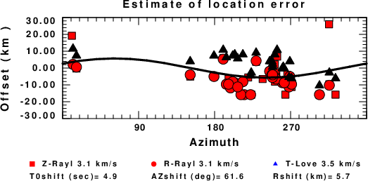
The derived shift in origin time and epicentral coordinates are given at the bottom of the figure.
Velocity Model
The CUS.model used for the waveform synthetic seismograms and for the surface wave eigenfunctions and dispersion is as follows
(The format is in the model96 format of Computer Programs in Seismology).
MODEL.01
CUS Model with Q from simple gamma values
ISOTROPIC
KGS
FLAT EARTH
1-D
CONSTANT VELOCITY
LINE08
LINE09
LINE10
LINE11
  H(KM) VP(KM/S) VS(KM/S) RHO(GM/CC)   QP   QS  ETAP  ETAS  FREFP  FREFS
  1.0000  5.0000  2.8900  2.5000 0.172E-02 0.387E-02 0.00  0.00  1.00  1.00
  9.0000  6.1000  3.5200  2.7300 0.160E-02 0.363E-02 0.00  0.00  1.00  1.00
 10.0000  6.4000  3.7000  2.8200 0.149E-02 0.336E-02 0.00  0.00  1.00  1.00
 20.0000  6.7000  3.8700  2.9020 0.000E-04 0.000E-04 0.00  0.00  1.00  1.00
  0.0000  8.1500  4.7000  3.3640 0.194E-02 0.431E-02 0.00  0.00  1.00  1.00
Last Changed Sun Jun 2 14:33:54 CDT 2024