The ANSS event ID is ak0246hfvypi and the event page is at https://earthquake.usgs.gov/earthquakes/eventpage/ak0246hfvypi/executive.
2024/05/20 15:30:34 67.970 -136.387 15.6 3.7 NWT, Canada
 USGS/SLU Moment Tensor Solution
 ENS  2024/05/20 15:30:34:0  67.97 -136.39  15.6 3.7 NWT, Canada

 Stations used:
   AK.C26K AK.C27K AK.COLD AK.D25K AK.DOT AK.E24K AK.E25K
   AK.E27K AK.G23K AK.G24K AK.GRES AK.H24K AK.HDA AK.I27K
   AK.J26L AK.POKR AK.PS04 AK.PS07 AK.PS08 AK.TOLK CN.CROWY
   CN.DAWY CN.INK CN.PAULN IU.COLA PQ.OGILY PQ.TSIIG US.EGAK

 Filtering commands used:
   cut o DIST/3.3 -30 o DIST/3.3 +80
   rtr
   taper w 0.1
   hp c 0.03 n 3
   lp c 0.10 n 3

 Best Fitting Double Couple
  Mo = 4.47e+21 dyne-cm
  Mw = 3.70
  Z  = 14 km
  Plane   Strike  Dip  Rake
   NP1        7    80   -129
   NP2      265    40   -15
  Principal Axes:
   Axis    Value   Plunge  Azimuth
    T   4.47e+21     25     126
    N   0.00e+00     38      14
    P  -4.47e+21     41     240

 Moment Tensor: (dyne-cm)
    Component   Value
       Mxx     6.48e+20
       Mxy    -2.83e+21
       Mxz     8.81e+19
       Myy     4.90e+20
       Myz     3.31e+21
       Mzz    -1.14e+21


                     ##########----
                 ##############--------
              #################-----------
             ##################------------
           #############-------###-----------
          #########------------#########------
         ######----------------############----
        #####------------------##############---
        ###--------------------################-
       ###---------------------#################-
       #-----------------------##################
       #----------------------###################
       -----------------------###################
        --------   -----------##################
        -------- P -----------##################
         -------   ----------##########   #####
          -------------------########## T ####
           -----------------###########   ###
             ---------------###############
              -------------###############
                 ----------############
                     -----#########


 Global CMT Convention Moment Tensor:
      R          T          P
 -1.14e+21   8.81e+19  -3.31e+21
  8.81e+19   6.48e+20   2.83e+21
 -3.31e+21   2.83e+21   4.90e+20


Details of the solution is found at

http://www.eas.slu.edu/eqc/eqc_mt/MECH.NA/20240520153034/index.html
|
      STK = 265
      DIP = 40
     RAKE = -15
       MW = 3.70
       HS = 14.0
The NDK file is 20240520153034.ndk I looed at the P waves and they were difficult to pick. The locaiton test indicates that the true local may be north of the AK locaiton. this may change the mechanism.
|
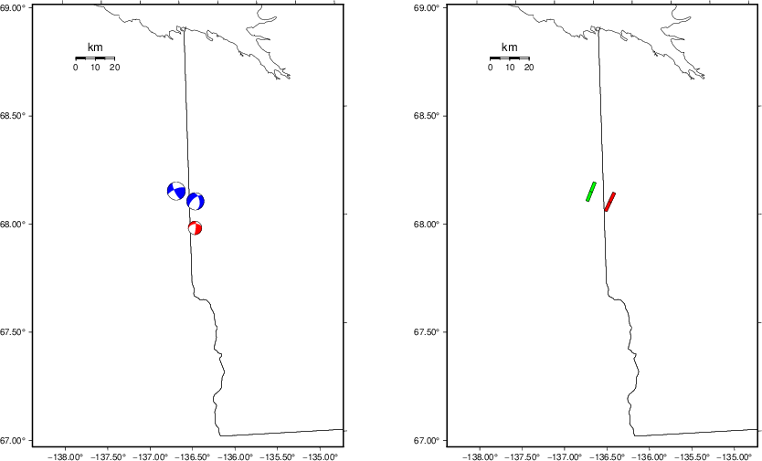
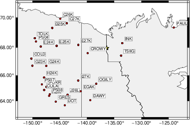
The focal mechanism was determined using broadband seismic waveforms. The location of the event (star) and the stations used for (red) the waveform inversion are shown in the next figure.
|
|
|
The program wvfgrd96 was used with good traces observed at short distance to determine the focal mechanism, depth and seismic moment. This technique requires a high quality signal and well determined velocity model for the Green's functions. To the extent that these are the quality data, this type of mechanism should be preferred over the radiation pattern technique which requires the separate step of defining the pressure and tension quadrants and the correct strike.
The observed and predicted traces are filtered using the following gsac commands:
cut o DIST/3.3 -30 o DIST/3.3 +80
rtr
taper w 0.1
hp c 0.03 n 3
lp c 0.10 n 3
The results of this grid search are as follow:
           DEPTH  STK   DIP  RAKE   MW    FIT
WVFGRD96    1.0    -5    40    85   3.33 0.3476
WVFGRD96    2.0   355    40    85   3.46 0.4026
WVFGRD96    3.0   110    25    30   3.51 0.3483
WVFGRD96    4.0   105    25    20   3.51 0.4230
WVFGRD96    5.0   105    30    20   3.52 0.4701
WVFGRD96    6.0   100    35    15   3.52 0.4986
WVFGRD96    7.0    95    40    10   3.53 0.5142
WVFGRD96    8.0    95    35     5   3.60 0.5246
WVFGRD96    9.0   265    35   -20   3.62 0.5450
WVFGRD96   10.0   265    40   -15   3.64 0.5687
WVFGRD96   11.0   265    40   -15   3.65 0.5858
WVFGRD96   12.0   265    40   -15   3.67 0.5966
WVFGRD96   13.0   265    40   -15   3.68 0.6031
WVFGRD96   14.0   265    40   -15   3.70 0.6052
WVFGRD96   15.0   265    40   -15   3.71 0.6043
WVFGRD96   16.0   265    40   -15   3.72 0.6004
WVFGRD96   17.0   265    40   -10   3.74 0.5944
WVFGRD96   18.0   265    40   -10   3.75 0.5862
WVFGRD96   19.0   265    40   -10   3.76 0.5756
WVFGRD96   20.0   265    40    -5   3.77 0.5639
WVFGRD96   21.0   265    40    -5   3.79 0.5509
WVFGRD96   22.0   265    35   -10   3.79 0.5368
WVFGRD96   23.0   270    35    -5   3.80 0.5226
WVFGRD96   24.0   270    35    -5   3.81 0.5077
WVFGRD96   25.0   265    35    -5   3.82 0.4919
WVFGRD96   26.0   270    30    -5   3.82 0.4754
WVFGRD96   27.0   270    30     0   3.83 0.4578
WVFGRD96   28.0   270    30     0   3.84 0.4390
WVFGRD96   29.0   270    30     0   3.84 0.4184
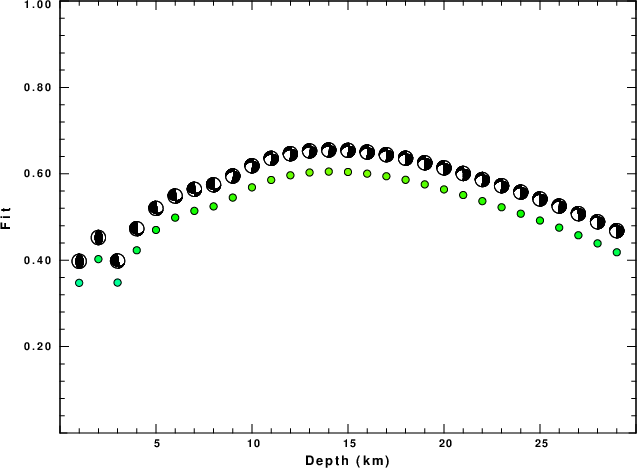
The best solution is
WVFGRD96 14.0 265 40 -15 3.70 0.6052
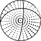
The mechanism corresponding to the best fit is
|
|
|
The best fit as a function of depth is given in the following figure:
|
|
|
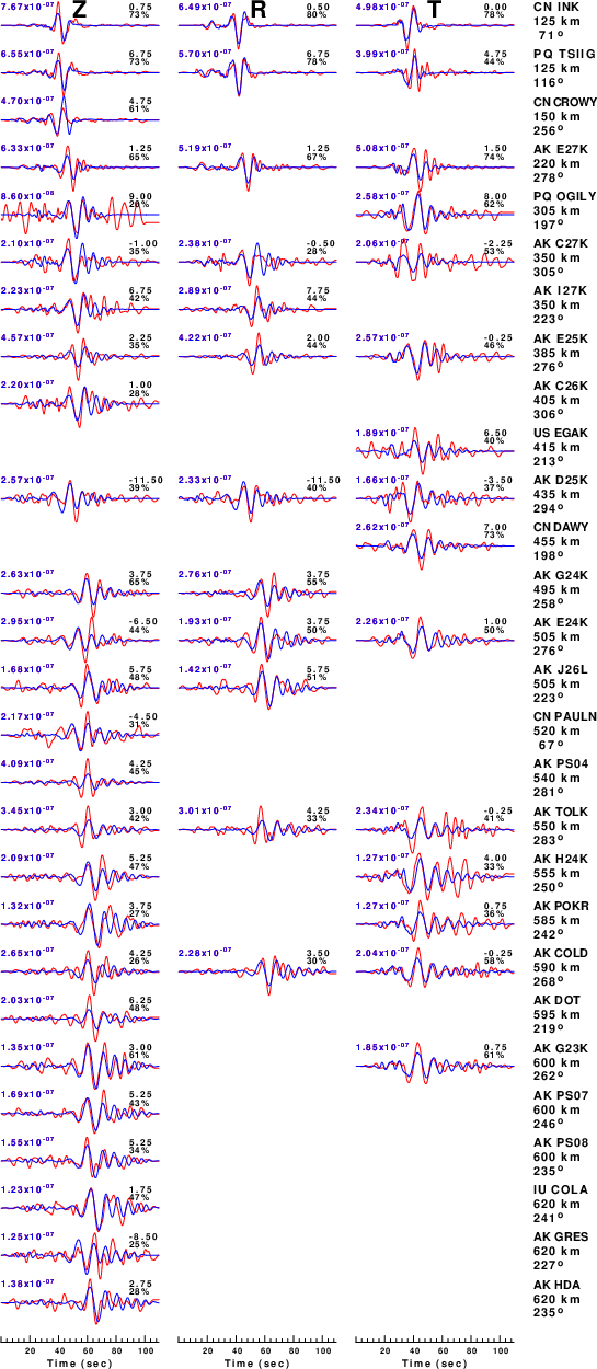
The comparison of the observed and predicted waveforms is given in the next figure. The red traces are the observed and the blue are the predicted. Each observed-predicted component is plotted to the same scale and peak amplitudes are indicated by the numbers to the left of each trace. A pair of numbers is given in black at the right of each predicted traces. The upper number it the time shift required for maximum correlation between the observed and predicted traces. This time shift is required because the synthetics are not computed at exactly the same distance as the observed, the velocity model used in the predictions may not be perfect and the epicentral parameters may be be off. A positive time shift indicates that the prediction is too fast and should be delayed to match the observed trace (shift to the right in this figure). A negative value indicates that the prediction is too slow. The lower number gives the percentage of variance reduction to characterize the individual goodness of fit (100% indicates a perfect fit).
The bandpass filter used in the processing and for the display was
cut o DIST/3.3 -30 o DIST/3.3 +80
rtr
taper w 0.1
hp c 0.03 n 3
lp c 0.10 n 3
|
| Figure 3. Waveform comparison for selected depth. Red: observed; Blue - predicted. The time shift with respect to the model prediction is indicated. The percent of fit is also indicated. The time scale is relative to the first trace sample. |
|
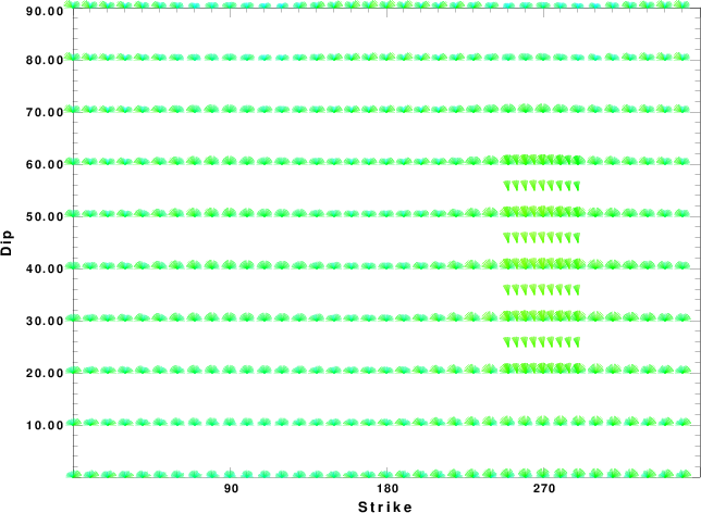
| Focal mechanism sensitivity at the preferred depth. The red color indicates a very good fit to the waveforms. Each solution is plotted as a vector at a given value of strike and dip with the angle of the vector representing the rake angle, measured, with respect to the upward vertical (N) in the figure. |
A check on the assumed source location is possible by looking at the time shifts between the observed and predicted traces. The time shifts for waveform matching arise for several reasons:
Time_shift = A + B cos Azimuth + C Sin Azimuth
The time shifts for this inversion lead to the next figure:
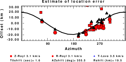
The derived shift in origin time and epicentral coordinates are given at the bottom of the figure.
The CUS.model used for the waveform synthetic seismograms and for the surface wave eigenfunctions and dispersion is as follows (The format is in the model96 format of Computer Programs in Seismology).
MODEL.01
CUS Model with Q from simple gamma values
ISOTROPIC
KGS
FLAT EARTH
1-D
CONSTANT VELOCITY
LINE08
LINE09
LINE10
LINE11
  H(KM) VP(KM/S) VS(KM/S) RHO(GM/CC)   QP   QS  ETAP  ETAS  FREFP  FREFS
  1.0000  5.0000  2.8900  2.5000 0.172E-02 0.387E-02 0.00  0.00  1.00  1.00
  9.0000  6.1000  3.5200  2.7300 0.160E-02 0.363E-02 0.00  0.00  1.00  1.00
 10.0000  6.4000  3.7000  2.8200 0.149E-02 0.336E-02 0.00  0.00  1.00  1.00
 20.0000  6.7000  3.8700  2.9020 0.000E-04 0.000E-04 0.00  0.00  1.00  1.00
  0.0000  8.1500  4.7000  3.3640 0.194E-02 0.431E-02 0.00  0.00  1.00  1.00