Location
Location ANSS
The ANSS event ID is ak023g35jxin and the event page is at
https://earthquake.usgs.gov/earthquakes/eventpage/ak023g35jxin/executive.
2023/12/16 19:24:39 60.248 -153.613 188.2 4.7 Alaska
Focal Mechanism
 USGS/SLU Moment Tensor Solution
 ENS  2023/12/16 19:24:39:0  60.25 -153.61 188.2 4.7 Alaska

 Stations used:
   AK.BAE AK.BRLK AK.CAST AK.CNP AK.CUT AK.FID AK.GHO AK.GLI
   AK.HIN AK.HOM AK.J19K AK.J20K AK.K20K AK.KLU AK.KNK AK.KTH
   AK.L20K AK.L22K AK.M16K AK.N15K AK.N18K AK.O14K AK.O18K
   AK.O19K AK.P16K AK.P17K AK.P23K AK.PPLA AK.RC01 AK.SAW
   AK.SCM AK.SKN AK.SLK AK.SWD AK.TRF AK.WAT6 AT.PMR AV.RED
   AV.STLK II.KDAK

 Filtering commands used:
   cut o DIST/3.7 -60 o DIST/3.7 +50
   rtr
   taper w 0.1
   hp c 0.03 n 3
   lp c 0.10 n 3

 Best Fitting Double Couple
  Mo = 9.66e+22 dyne-cm
  Mw = 4.59
  Z  = 202 km
  Plane   Strike  Dip  Rake
   NP1        5    80    75
   NP2      242    18   146
  Principal Axes:
   Axis    Value   Plunge  Azimuth
    T   9.66e+22     53     257
    N   0.00e+00     15       8
    P  -9.66e+22     33     108

 Moment Tensor: (dyne-cm)
    Component   Value
       Mxx    -4.52e+21
       Mxy     2.70e+22
       Mxz     3.32e+21
       Myy    -2.74e+22
       Myz    -8.77e+22
       Mzz     3.19e+22


                     ---------#####
                 ----------###---######
              -------##########--------###
             -----#############-----------#
           ----################-------------#
          ----#################---------------
         ---###################----------------
        ---####################-----------------
        --#####################-----------------
       ---#####################------------------
       --######################------------------
       --########   ##########-------------------
       --######## T ##########----------   ------
        -########   ##########---------- P -----
        -#####################----------   -----
         #####################-----------------
          ###################-----------------
           ##################----------------
             ###############---------------
              ##############--------------
                 ##########------------
                     ######--------


 Global CMT Convention Moment Tensor:
      R          T          P
  3.19e+22   3.32e+21   8.77e+22
  3.32e+21  -4.52e+21  -2.70e+22
  8.77e+22  -2.70e+22  -2.74e+22


Details of the solution is found at

http://www.eas.slu.edu/eqc/eqc_mt/MECH.NA/20231216192439/index.html
|
Preferred Solution
The preferred solution from an analysis of the surface-wave spectral amplitude radiation pattern, waveform inversion or first motion observations is
      STK = 5
      DIP = 80
     RAKE = 75
       MW = 4.59
       HS = 202.0
The NDK file is 20231216192439.ndk
The waveform inversion is preferred.
Moment Tensor Comparison
The following compares this source inversion to those provided by others. The purpose is to look for major differences and also to note slight differences that might be inherent to the processing procedure. For completeness the USGS/SLU solution is repeated from above.
| SLU |
USGSW |
 USGS/SLU Moment Tensor Solution
 ENS  2023/12/16 19:24:39:0  60.25 -153.61 188.2 4.7 Alaska

 Stations used:
   AK.BAE AK.BRLK AK.CAST AK.CNP AK.CUT AK.FID AK.GHO AK.GLI
   AK.HIN AK.HOM AK.J19K AK.J20K AK.K20K AK.KLU AK.KNK AK.KTH
   AK.L20K AK.L22K AK.M16K AK.N15K AK.N18K AK.O14K AK.O18K
   AK.O19K AK.P16K AK.P17K AK.P23K AK.PPLA AK.RC01 AK.SAW
   AK.SCM AK.SKN AK.SLK AK.SWD AK.TRF AK.WAT6 AT.PMR AV.RED
   AV.STLK II.KDAK

 Filtering commands used:
   cut o DIST/3.7 -60 o DIST/3.7 +50
   rtr
   taper w 0.1
   hp c 0.03 n 3
   lp c 0.10 n 3

 Best Fitting Double Couple
  Mo = 9.66e+22 dyne-cm
  Mw = 4.59
  Z  = 202 km
  Plane   Strike  Dip  Rake
   NP1        5    80    75
   NP2      242    18   146
  Principal Axes:
   Axis    Value   Plunge  Azimuth
    T   9.66e+22     53     257
    N   0.00e+00     15       8
    P  -9.66e+22     33     108

 Moment Tensor: (dyne-cm)
    Component   Value
       Mxx    -4.52e+21
       Mxy     2.70e+22
       Mxz     3.32e+21
       Myy    -2.74e+22
       Myz    -8.77e+22
       Mzz     3.19e+22


                     ---------#####
                 ----------###---######
              -------##########--------###
             -----#############-----------#
           ----################-------------#
          ----#################---------------
         ---###################----------------
        ---####################-----------------
        --#####################-----------------
       ---#####################------------------
       --######################------------------
       --########   ##########-------------------
       --######## T ##########----------   ------
        -########   ##########---------- P -----
        -#####################----------   -----
         #####################-----------------
          ###################-----------------
           ##################----------------
             ###############---------------
              ##############--------------
                 ##########------------
                     ######--------


 Global CMT Convention Moment Tensor:
      R          T          P
  3.19e+22   3.32e+21   8.77e+22
  3.32e+21  -4.52e+21  -2.70e+22
  8.77e+22  -2.70e+22  -2.74e+22


Details of the solution is found at

http://www.eas.slu.edu/eqc/eqc_mt/MECH.NA/20231216192439/index.html
|
W-phase Moment Tensor (Mww)
Moment
1.607e+16 N-m
Magnitude
4.74 Mww
Depth
180.5 km
Percent DC
60%
Half Duration
0.61 s
Catalog
US
Data Source
US 3
Contributor
US 3
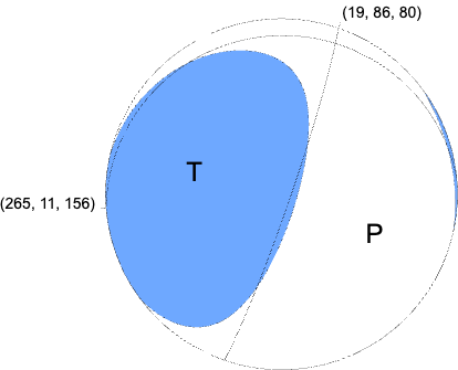
Nodal Planes
Plane Strike Dip Rake
NP1 265 11 156
NP2 19 86 80
Principal Axes
Axis Value Plunge Azimuth
T 1.753e+16 48 279
N -0.349e+16 10 20
P -1.404e+16 40 118
|
Magnitudes
Given the availability of digital waveforms for determination of the moment tensor, this section documents the added processing leading to mLg, if appropriate to the region, and ML by application of the respective IASPEI formulae. As a research study, the linear distance term of the IASPEI formula
for ML is adjusted to remove a linear distance trend in residuals to give a regionally defined ML. The defined ML uses horizontal component recordings, but the same procedure is applied to the vertical components since there may be some interest in vertical component ground motions. Residual plots versus distance may indicate interesting features of ground motion scaling in some distance ranges. A residual plot of the regionalized magnitude is given as a function of distance and azimuth, since data sets may transcend different wave propagation provinces.
ML Magnitude
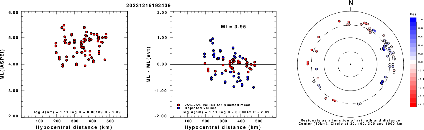
Left: ML computed using the IASPEI formula for Horizontal components. Center: ML residuals computed using a modified IASPEI formula that accounts for path specific attenuation; the values used for the trimmed mean are indicated. The ML relation used for each figure is given at the bottom of each plot.
Right: Residuals from new relation as a function of distance and azimuth.
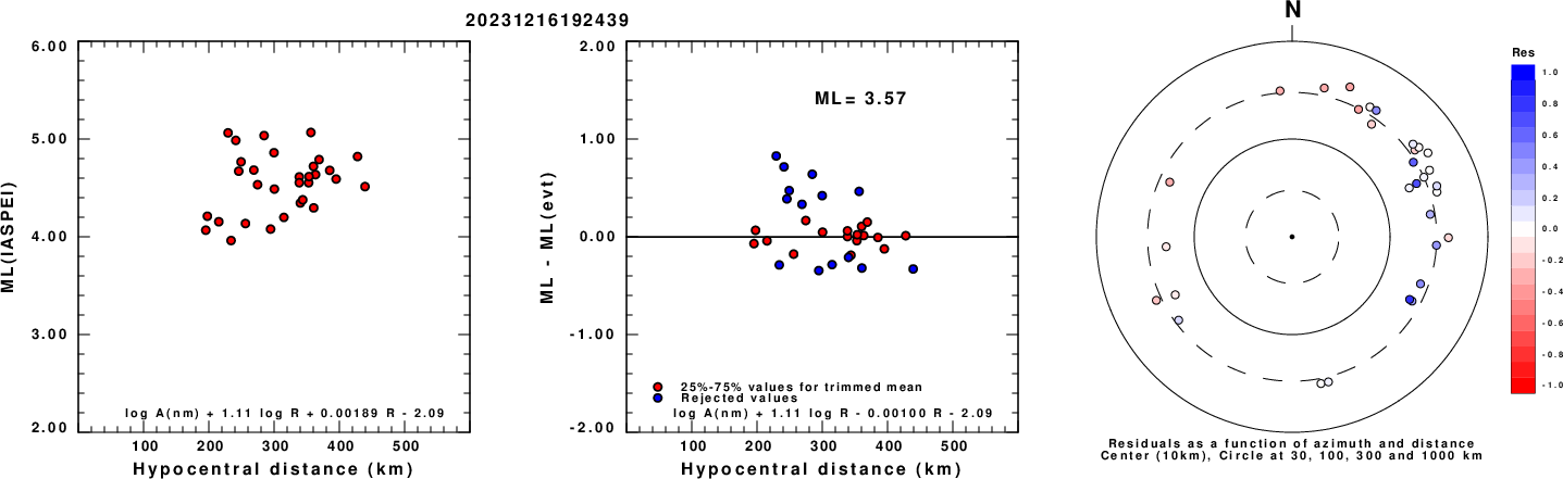
Left: ML computed using the IASPEI formula for Vertical components (research). Center: ML residuals computed using a modified IASPEI formula that accounts for path specific attenuation; the values used for the trimmed mean are indicated. The ML relation used for each figure is given at the bottom of each plot.
Right: Residuals from new relation as a function of distance and azimuth.
Context
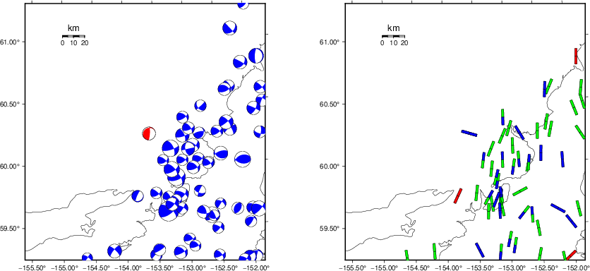
The left panel of the next figure presents the focal mechanism for this earthquake (red) in the context of other nearby events (blue) in the SLU Moment Tensor Catalog. The right panel shows the inferred direction of maximum compressive stress and the type of faulting (green is strike-slip, red is normal, blue is thrust; oblique is shown by a combination of colors). Thus context plot is useful for assessing the appropriateness of the moment tensor of this event.
Waveform Inversion using wvfgrd96
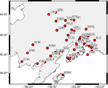
The focal mechanism was determined using broadband seismic waveforms. The location of the event (star) and the
stations used for (red) the waveform inversion are shown in the next figure.
|
|
Location of broadband stations used for waveform inversion
|
The program wvfgrd96 was used with good traces observed at short distance to determine the focal mechanism, depth and seismic moment. This technique requires a high quality signal and well determined velocity model for the Green's functions. To the extent that these are the quality data, this type of mechanism should be preferred over the radiation pattern technique which requires the separate step of defining the pressure and tension quadrants and the correct strike.
The observed and predicted traces are filtered using the following gsac commands:
cut o DIST/3.7 -60 o DIST/3.7 +50
rtr
taper w 0.1
hp c 0.03 n 3
lp c 0.10 n 3
The results of this grid search are as follow:
           DEPTH  STK   DIP  RAKE   MW    FIT
WVFGRD96  100.0   255    55   -70   4.29 0.1367
WVFGRD96  102.0   250    55   -75   4.29 0.1400
WVFGRD96  104.0   255    55   -70   4.30 0.1440
WVFGRD96  106.0   255    55   -70   4.31 0.1503
WVFGRD96  108.0   250    50   -60   4.31 0.1568
WVFGRD96  110.0   250    50   -55   4.32 0.1632
WVFGRD96  112.0   250    50   -55   4.32 0.1686
WVFGRD96  114.0   250    50   -55   4.33 0.1723
WVFGRD96  116.0   250    50   -55   4.33 0.1745
WVFGRD96  118.0   215    70    50   4.41 0.1846
WVFGRD96  120.0   220    65    50   4.42 0.2021
WVFGRD96  122.0   225    60    55   4.42 0.2208
WVFGRD96  124.0    55    45    55   4.38 0.2501
WVFGRD96  126.0    55    45    55   4.40 0.2856
WVFGRD96  128.0    55    45    55   4.42 0.3232
WVFGRD96  130.0    55    45    55   4.43 0.3627
WVFGRD96  132.0    55    45    55   4.45 0.4137
WVFGRD96  134.0    25    60    55   4.48 0.4520
WVFGRD96  136.0    20    65    55   4.49 0.4873
WVFGRD96  138.0    20    65    55   4.50 0.5226
WVFGRD96  140.0    20    65    55   4.51 0.5387
WVFGRD96  142.0    15    70    55   4.52 0.5474
WVFGRD96  144.0    15    70    55   4.52 0.5524
WVFGRD96  146.0    15    70    55   4.52 0.5567
WVFGRD96  148.0    15    70    55   4.52 0.5619
WVFGRD96  150.0    15    70    55   4.53 0.5663
WVFGRD96  152.0    15    70    55   4.53 0.5694
WVFGRD96  154.0    15    70    55   4.53 0.5747
WVFGRD96  156.0    15    70    55   4.53 0.5785
WVFGRD96  158.0    15    70    55   4.54 0.5815
WVFGRD96  160.0    15    70    55   4.54 0.5869
WVFGRD96  162.0    15    70    55   4.54 0.5902
WVFGRD96  164.0    15    70    55   4.54 0.5938
WVFGRD96  166.0    15    70    55   4.55 0.5977
WVFGRD96  168.0    15    70    55   4.55 0.6015
WVFGRD96  170.0    15    70    55   4.55 0.6044
WVFGRD96  162.0    15    70    55   4.54 0.5902
WVFGRD96  164.0    15    70    55   4.54 0.5938
WVFGRD96  166.0    15    70    55   4.55 0.5977
WVFGRD96  168.0    15    70    55   4.55 0.6015
WVFGRD96  180.0     5    80    70   4.57 0.6211
WVFGRD96  182.0     5    80    70   4.57 0.6247
WVFGRD96  184.0     5    80    70   4.57 0.6309
WVFGRD96  186.0     5    80    70   4.57 0.6344
WVFGRD96  188.0     5    80    70   4.58 0.6381
WVFGRD96  190.0     5    80    70   4.58 0.6426
WVFGRD96  192.0     5    80    70   4.58 0.6457
WVFGRD96  194.0     5    80    70   4.58 0.6486
WVFGRD96  196.0     5    80    75   4.58 0.6511
WVFGRD96  198.0     5    80    75   4.58 0.6536
WVFGRD96  200.0     5    80    75   4.59 0.6548
WVFGRD96  202.0     5    80    75   4.59 0.6565
WVFGRD96  204.0     5    80    75   4.59 0.6561
WVFGRD96  206.0     5    80    75   4.59 0.6558
WVFGRD96  208.0     5    80    75   4.59 0.6540
The best solution is
WVFGRD96 202.0 5 80 75 4.59 0.6565
The mechanism corresponding to the best fit is
|
|
Figure 1. Waveform inversion focal mechanism
|
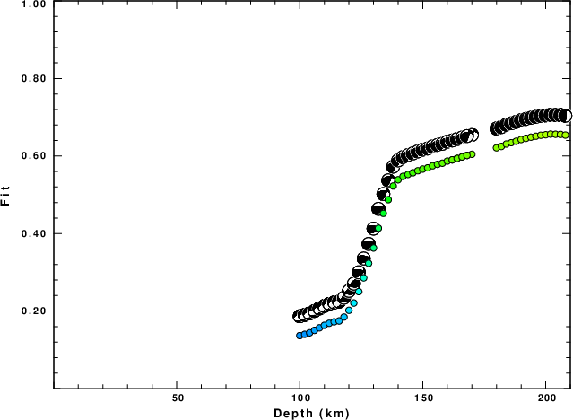
The best fit as a function of depth is given in the following figure:
|
|
Figure 2. Depth sensitivity for waveform mechanism
|
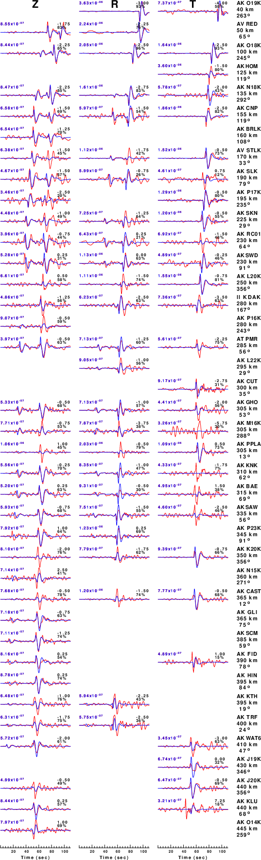
The comparison of the observed and predicted waveforms is given in the next figure. The red traces are the observed and the blue are the predicted.
Each observed-predicted component is plotted to the same scale and peak amplitudes are indicated by the numbers to the left of each trace. A pair of numbers is given in black at the right of each predicted traces. The upper number it the time shift required for maximum correlation between the observed and predicted traces. This time shift is required because the synthetics are not computed at exactly the same distance as the observed, the velocity model used in the predictions may not be perfect and the epicentral parameters may be be off.
A positive time shift indicates that the prediction is too fast and should be delayed to match the observed trace (shift to the right in this figure). A negative value indicates that the prediction is too slow. The lower number gives the percentage of variance reduction to characterize the individual goodness of fit (100% indicates a perfect fit).
The bandpass filter used in the processing and for the display was
cut o DIST/3.7 -60 o DIST/3.7 +50
rtr
taper w 0.1
hp c 0.03 n 3
lp c 0.10 n 3
|
|
Figure 3. Waveform comparison for selected depth. Red: observed; Blue - predicted. The time shift with respect to the model prediction is indicated. The percent of fit is also indicated. The time scale is relative to the first trace sample.
|
|
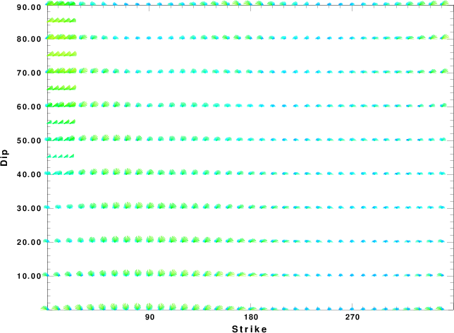
|
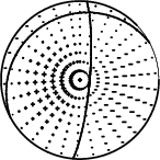
Focal mechanism sensitivity at the preferred depth. The red color indicates a very good fit to the waveforms.
Each solution is plotted as a vector at a given value of strike and dip with the angle of the vector representing the rake angle, measured, with respect to the upward vertical (N) in the figure.
|
A check on the assumed source location is possible by looking at the time shifts between the observed and predicted traces. The time shifts for waveform matching arise for several reasons:
- The origin time and epicentral distance are incorrect
- The velocity model used for the inversion is incorrect
- The velocity model used to define the P-arrival time is not the
same as the velocity model used for the waveform inversion
(assuming that the initial trace alignment is based on the
P arrival time)
Assuming only a mislocation, the time shifts are fit to a functional form:
Time_shift = A + B cos Azimuth + C Sin Azimuth
The time shifts for this inversion lead to the next figure:
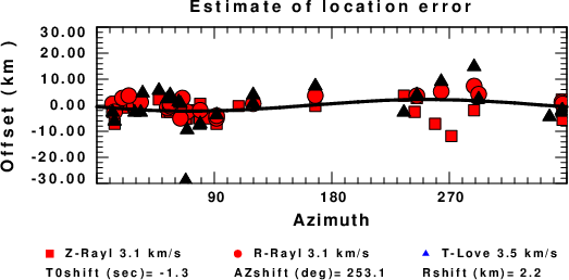
The derived shift in origin time and epicentral coordinates are given at the bottom of the figure.
Velocity Model
The WUS.model used for the waveform synthetic seismograms and for the surface wave eigenfunctions and dispersion is as follows
(The format is in the model96 format of Computer Programs in Seismology).
MODEL.01
Model after     8 iterations
ISOTROPIC
KGS
FLAT EARTH
1-D
CONSTANT VELOCITY
LINE08
LINE09
LINE10
LINE11
      H(KM)   VP(KM/S)   VS(KM/S) RHO(GM/CC)         QP         QS       ETAP       ETAS      FREFP      FREFS
     1.9000     3.4065     2.0089     2.2150  0.302E-02  0.679E-02   0.00       0.00       1.00       1.00
     6.1000     5.5445     3.2953     2.6089  0.349E-02  0.784E-02   0.00       0.00       1.00       1.00
    13.0000     6.2708     3.7396     2.7812  0.212E-02  0.476E-02   0.00       0.00       1.00       1.00
    19.0000     6.4075     3.7680     2.8223  0.111E-02  0.249E-02   0.00       0.00       1.00       1.00
     0.0000     7.9000     4.6200     3.2760  0.164E-10  0.370E-10   0.00       0.00       1.00       1.00
Last Changed Tue Apr 23 06:26:43 AM CDT 2024