Location
Location ANSS
The ANSS event ID is ak023fe4b796 and the event page is at
https://earthquake.usgs.gov/earthquakes/eventpage/ak023fe4b796/executive.
2023/12/01 05:50:26 62.957 -150.435 101.7 5.1 Alaska
Focal Mechanism
 USGS/SLU Moment Tensor Solution
 ENS  2023/12/01 05:50:26:0  62.96 -150.43 101.7 5.1 Alaska

 Stations used:
   AK.BAE AK.BPAW AK.CAST AK.CCB AK.CUT AK.DHY AK.DOT AK.GHO
   AK.H21K AK.HDA AK.I21K AK.I23K AK.J19K AK.J20K AK.K20K
   AK.K24K AK.KNK AK.L20K AK.L22K AK.M20K AK.MCK AK.MLY
   AK.NEA2 AK.PAX AK.POKR AK.PPLA AK.PWL AK.RC01 AK.RND AK.SAW
   AK.SCM AK.SCRK AK.SKN AK.TRF AK.WAT6 AK.WRH AT.PMR AV.STLK
   IM.IL31 IU.COLA

 Filtering commands used:
   cut o DIST/3.3 -60 o DIST/3.3 +30
   rtr
   taper w 0.1
   hp c 0.03 n 3
   lp c 0.08 n 3

 Best Fitting Double Couple
  Mo = 4.27e+23 dyne-cm
  Mw = 5.02
  Z  = 106 km
  Plane   Strike  Dip  Rake
   NP1      336    71   126
   NP2       90    40    30
  Principal Axes:
   Axis    Value   Plunge  Azimuth
    T   4.27e+23     50     287
    N   0.00e+00     34     143
    P  -4.27e+23     18      40

 Moment Tensor: (dyne-cm)
    Component   Value
       Mxx    -2.10e+23
       Mxy    -2.37e+23
       Mxz    -3.70e+22
       Myy    -2.08e+16
       Myz    -2.83e+23
       Mzz     2.10e+23


                     --------------
                 #####-----------------
              ##########-------------   --
             ############------------ P ---
           ################----------   -----
          ##################------------------
         ####################------------------
        ######################------------------
        #########   ###########-----------------
       ########## T ############-----------------
       ##########   #############----------------
       -##########################--------------#
       --#########################-------------##
        --#########################-----------##
        ----#######################---------####
         -----######################------#####
          --------##################--########
           -------------########----#########
             ------------------------######
              -----------------------#####
                 --------------------##
                     --------------


 Global CMT Convention Moment Tensor:
      R          T          P
  2.10e+23  -3.70e+22   2.83e+23
 -3.70e+22  -2.10e+23   2.37e+23
  2.83e+23   2.37e+23  -2.08e+16


Details of the solution is found at

http://www.eas.slu.edu/eqc/eqc_mt/MECH.NA/20231201055026/index.html
|
Preferred Solution
The preferred solution from an analysis of the surface-wave spectral amplitude radiation pattern, waveform inversion or first motion observations is
      STK = 90
      DIP = 40
     RAKE = 30
       MW = 5.02
       HS = 106.0
The NDK file is 20231201055026.ndk
The waveform inversion is preferred.
Moment Tensor Comparison
The following compares this source inversion to those provided by others. The purpose is to look for major differences and also to note slight differences that might be inherent to the processing procedure. For completeness the USGS/SLU solution is repeated from above.
| SLU |
USGSMWR |
USGSW |
 USGS/SLU Moment Tensor Solution
 ENS  2023/12/01 05:50:26:0  62.96 -150.43 101.7 5.1 Alaska

 Stations used:
   AK.BAE AK.BPAW AK.CAST AK.CCB AK.CUT AK.DHY AK.DOT AK.GHO
   AK.H21K AK.HDA AK.I21K AK.I23K AK.J19K AK.J20K AK.K20K
   AK.K24K AK.KNK AK.L20K AK.L22K AK.M20K AK.MCK AK.MLY
   AK.NEA2 AK.PAX AK.POKR AK.PPLA AK.PWL AK.RC01 AK.RND AK.SAW
   AK.SCM AK.SCRK AK.SKN AK.TRF AK.WAT6 AK.WRH AT.PMR AV.STLK
   IM.IL31 IU.COLA

 Filtering commands used:
   cut o DIST/3.3 -60 o DIST/3.3 +30
   rtr
   taper w 0.1
   hp c 0.03 n 3
   lp c 0.08 n 3

 Best Fitting Double Couple
  Mo = 4.27e+23 dyne-cm
  Mw = 5.02
  Z  = 106 km
  Plane   Strike  Dip  Rake
   NP1      336    71   126
   NP2       90    40    30
  Principal Axes:
   Axis    Value   Plunge  Azimuth
    T   4.27e+23     50     287
    N   0.00e+00     34     143
    P  -4.27e+23     18      40

 Moment Tensor: (dyne-cm)
    Component   Value
       Mxx    -2.10e+23
       Mxy    -2.37e+23
       Mxz    -3.70e+22
       Myy    -2.08e+16
       Myz    -2.83e+23
       Mzz     2.10e+23


                     --------------
                 #####-----------------
              ##########-------------   --
             ############------------ P ---
           ################----------   -----
          ##################------------------
         ####################------------------
        ######################------------------
        #########   ###########-----------------
       ########## T ############-----------------
       ##########   #############----------------
       -##########################--------------#
       --#########################-------------##
        --#########################-----------##
        ----#######################---------####
         -----######################------#####
          --------##################--########
           -------------########----#########
             ------------------------######
              -----------------------#####
                 --------------------##
                     --------------


 Global CMT Convention Moment Tensor:
      R          T          P
  2.10e+23  -3.70e+22   2.83e+23
 -3.70e+22  -2.10e+23   2.37e+23
  2.83e+23   2.37e+23  -2.08e+16


Details of the solution is found at

http://www.eas.slu.edu/eqc/eqc_mt/MECH.NA/20231201055026/index.html
|
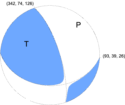
Regional Moment Tensor (Mwr)
Moment
4.838e+16 N-m
Magnitude
5.06 Mwr
Depth
102.0 km
Percent DC
97%
Half Duration
-
Catalog
US
Data Source
US 3
Contributor
US 3
Nodal Planes
Plane	Strike	Dip	Rake
NP1	342	74	126
NP2	93	39	26
Principal Axes
Axis	Value	Plunge	Azimuth
T	4.879e+16	48	290
N	-0.083e+16	34	151
P	-4.796e+16	21	46
|
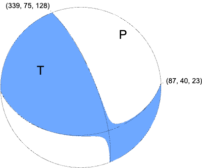
W-phase Moment Tensor (Mww)
Moment
4.620e+16 N-m
Magnitude
5.04 Mww
Depth
100.5 km
Percent DC
96%
Half Duration
0.86 s
Catalog
US
Data Source
US 3
Contributor
US 3
Nodal Planes
Plane	Strike	Dip	Rake
NP1	339	75	128
NP2	87	40	23
Principal Axes
Axis	Value	Plunge	Azimuth
T	4.569e+16	46	287
N	0.099e+16	36	147
P	-4.668e+16	21	41
|
Magnitudes
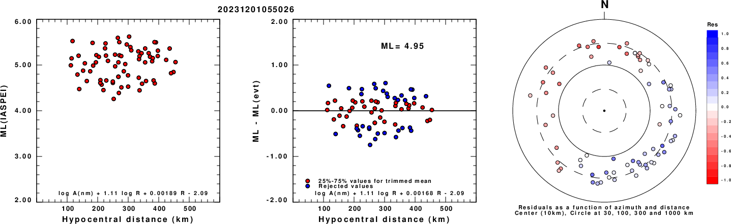
Given the availability of digital waveforms for determination of the moment tensor, this section documents the added processing leading to mLg, if appropriate to the region, and ML by application of the respective IASPEI formulae. As a research study, the linear distance term of the IASPEI formula
for ML is adjusted to remove a linear distance trend in residuals to give a regionally defined ML. The defined ML uses horizontal component recordings, but the same procedure is applied to the vertical components since there may be some interest in vertical component ground motions. Residual plots versus distance may indicate interesting features of ground motion scaling in some distance ranges. A residual plot of the regionalized magnitude is given as a function of distance and azimuth, since data sets may transcend different wave propagation provinces.
ML Magnitude
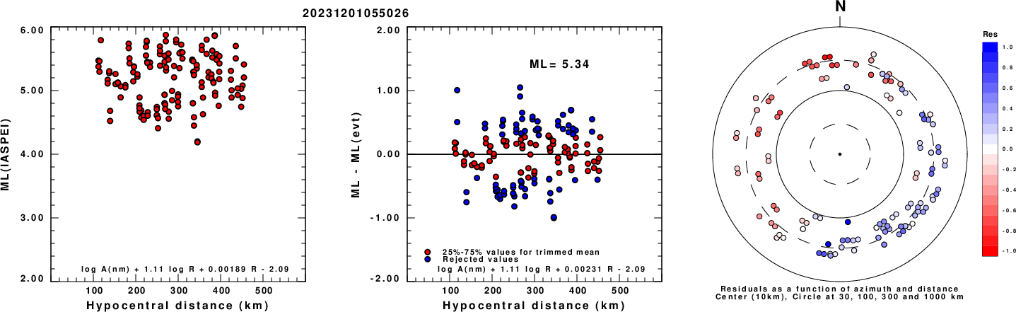
Left: ML computed using the IASPEI formula for Horizontal components. Center: ML residuals computed using a modified IASPEI formula that accounts for path specific attenuation; the values used for the trimmed mean are indicated. The ML relation used for each figure is given at the bottom of each plot.
Right: Residuals from new relation as a function of distance and azimuth.
Left: ML computed using the IASPEI formula for Vertical components (research). Center: ML residuals computed using a modified IASPEI formula that accounts for path specific attenuation; the values used for the trimmed mean are indicated. The ML relation used for each figure is given at the bottom of each plot.
Right: Residuals from new relation as a function of distance and azimuth.
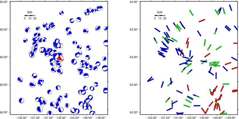
Context
The left panel of the next figure presents the focal mechanism for this earthquake (red) in the context of other nearby events (blue) in the SLU Moment Tensor Catalog. The right panel shows the inferred direction of maximum compressive stress and the type of faulting (green is strike-slip, red is normal, blue is thrust; oblique is shown by a combination of colors). Thus context plot is useful for assessing the appropriateness of the moment tensor of this event.
Waveform Inversion using wvfgrd96
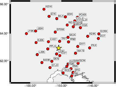
The focal mechanism was determined using broadband seismic waveforms. The location of the event (star) and the
stations used for (red) the waveform inversion are shown in the next figure.
|
|
Location of broadband stations used for waveform inversion
|
The program wvfgrd96 was used with good traces observed at short distance to determine the focal mechanism, depth and seismic moment. This technique requires a high quality signal and well determined velocity model for the Green's functions. To the extent that these are the quality data, this type of mechanism should be preferred over the radiation pattern technique which requires the separate step of defining the pressure and tension quadrants and the correct strike.
The observed and predicted traces are filtered using the following gsac commands:
cut o DIST/3.3 -60 o DIST/3.3 +30
rtr
taper w 0.1
hp c 0.03 n 3
lp c 0.08 n 3
The results of this grid search are as follow:
           DEPTH  STK   DIP  RAKE   MW    FIT
WVFGRD96    2.0   145    55   -65   4.18 0.2734
WVFGRD96    4.0   145    80   -45   4.22 0.2618
WVFGRD96    6.0   150    90   -40   4.25 0.2924
WVFGRD96    8.0   330    85    40   4.32 0.3173
WVFGRD96   10.0   145    80   -35   4.36 0.3376
WVFGRD96   12.0   145    80   -35   4.39 0.3502
WVFGRD96   14.0   145    80   -30   4.41 0.3534
WVFGRD96   16.0   145    80   -30   4.43 0.3502
WVFGRD96   18.0   145    80   -30   4.45 0.3425
WVFGRD96   20.0   145    80   -30   4.46 0.3314
WVFGRD96   22.0   140    75   -35   4.48 0.3190
WVFGRD96   24.0   240    55    15   4.49 0.3075
WVFGRD96   26.0   245    55    20   4.51 0.3126
WVFGRD96   28.0   245    55    20   4.53 0.3184
WVFGRD96   30.0    90    65    25   4.56 0.3248
WVFGRD96   32.0    95    60    30   4.58 0.3364
WVFGRD96   34.0    90    65    25   4.60 0.3458
WVFGRD96   36.0    75    70    20   4.64 0.3549
WVFGRD96   38.0    90    65    30   4.65 0.3620
WVFGRD96   40.0    90    65    35   4.73 0.3808
WVFGRD96   42.0    90    65    35   4.75 0.3869
WVFGRD96   44.0    80    65    30   4.78 0.3919
WVFGRD96   46.0    80    60    30   4.80 0.3995
WVFGRD96   48.0    80    60    25   4.82 0.4104
WVFGRD96   50.0    90    55    30   4.83 0.4261
WVFGRD96   52.0    90    55    30   4.85 0.4448
WVFGRD96   54.0    90    50    30   4.86 0.4645
WVFGRD96   56.0    90    50    30   4.88 0.4896
WVFGRD96   58.0    90    50    30   4.89 0.5155
WVFGRD96   60.0    90    50    30   4.90 0.5414
WVFGRD96   62.0    90    45    25   4.92 0.5663
WVFGRD96   64.0    90    45    25   4.93 0.5901
WVFGRD96   66.0    85    45    25   4.93 0.6145
WVFGRD96   68.0    85    45    25   4.94 0.6369
WVFGRD96   70.0    85    40    25   4.95 0.6576
WVFGRD96   72.0    85    40    20   4.96 0.6780
WVFGRD96   74.0    85    40    20   4.97 0.6950
WVFGRD96   76.0    85    40    20   4.98 0.7108
WVFGRD96   78.0    85    40    20   4.98 0.7256
WVFGRD96   80.0    85    40    20   4.99 0.7376
WVFGRD96   82.0    85    40    20   4.99 0.7493
WVFGRD96   84.0    85    40    20   4.99 0.7594
WVFGRD96   86.0    85    40    25   4.99 0.7684
WVFGRD96   88.0    90    40    30   4.99 0.7772
WVFGRD96   90.0    90    40    30   5.00 0.7866
WVFGRD96   92.0    90    40    30   5.00 0.7948
WVFGRD96   94.0    90    40    30   5.00 0.8025
WVFGRD96   96.0    90    40    30   5.01 0.8081
WVFGRD96   98.0    90    40    30   5.01 0.8135
WVFGRD96  100.0    90    40    30   5.01 0.8168
WVFGRD96  102.0    90    40    30   5.02 0.8208
WVFGRD96  104.0    90    40    30   5.02 0.8224
WVFGRD96  106.0    90    40    30   5.02 0.8239
WVFGRD96  108.0    90    40    30   5.02 0.8225
WVFGRD96  110.0    90    40    30   5.03 0.8224
WVFGRD96  112.0    90    40    30   5.03 0.8201
WVFGRD96  114.0    90    40    30   5.03 0.8182
WVFGRD96  116.0    90    40    30   5.03 0.8138
WVFGRD96  118.0    90    40    30   5.03 0.8104
WVFGRD96  120.0    90    40    30   5.03 0.8040
WVFGRD96  122.0    90    40    30   5.04 0.7990
WVFGRD96  124.0    90    40    30   5.04 0.7919
WVFGRD96  126.0    90    45    25   5.04 0.7854
WVFGRD96  128.0    90    45    25   5.04 0.7781
WVFGRD96  130.0    90    45    25   5.05 0.7713
WVFGRD96  132.0    90    45    25   5.05 0.7640
WVFGRD96  134.0    90    45    25   5.05 0.7560
WVFGRD96  136.0    90    45    25   5.05 0.7500
WVFGRD96  138.0    90    45    30   5.04 0.7432
WVFGRD96  140.0    90    45    30   5.05 0.7373
WVFGRD96  142.0    90    45    30   5.05 0.7322
WVFGRD96  144.0    90    45    30   5.05 0.7266
WVFGRD96  146.0    90    45    30   5.05 0.7217
WVFGRD96  148.0    90    45    30   5.05 0.7155
The best solution is
WVFGRD96 106.0 90 40 30 5.02 0.8239
The mechanism corresponding to the best fit is
|
|
Figure 1. Waveform inversion focal mechanism
|
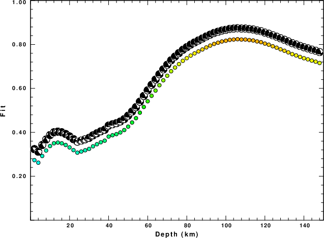
The best fit as a function of depth is given in the following figure:
|
|
Figure 2. Depth sensitivity for waveform mechanism
|
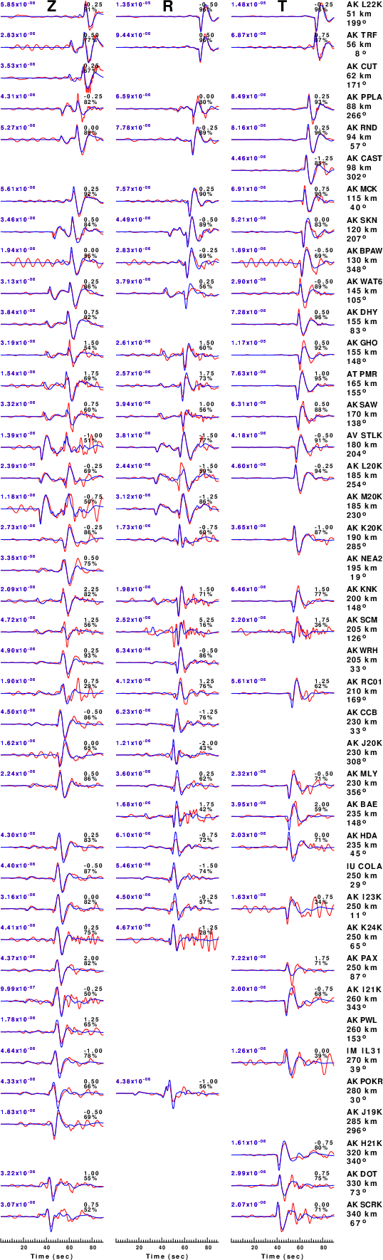
The comparison of the observed and predicted waveforms is given in the next figure. The red traces are the observed and the blue are the predicted.
Each observed-predicted component is plotted to the same scale and peak amplitudes are indicated by the numbers to the left of each trace. A pair of numbers is given in black at the right of each predicted traces. The upper number it the time shift required for maximum correlation between the observed and predicted traces. This time shift is required because the synthetics are not computed at exactly the same distance as the observed, the velocity model used in the predictions may not be perfect and the epicentral parameters may be be off.
A positive time shift indicates that the prediction is too fast and should be delayed to match the observed trace (shift to the right in this figure). A negative value indicates that the prediction is too slow. The lower number gives the percentage of variance reduction to characterize the individual goodness of fit (100% indicates a perfect fit).
The bandpass filter used in the processing and for the display was
cut o DIST/3.3 -60 o DIST/3.3 +30
rtr
taper w 0.1
hp c 0.03 n 3
lp c 0.08 n 3
|
|
Figure 3. Waveform comparison for selected depth. Red: observed; Blue - predicted. The time shift with respect to the model prediction is indicated. The percent of fit is also indicated. The time scale is relative to the first trace sample.
|
|
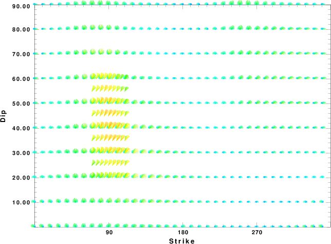
|
Focal mechanism sensitivity at the preferred depth. The red color indicates a very good fit to the waveforms.
Each solution is plotted as a vector at a given value of strike and dip with the angle of the vector representing the rake angle, measured, with respect to the upward vertical (N) in the figure.
|
A check on the assumed source location is possible by looking at the time shifts between the observed and predicted traces. The time shifts for waveform matching arise for several reasons:
- The origin time and epicentral distance are incorrect
- The velocity model used for the inversion is incorrect
- The velocity model used to define the P-arrival time is not the
same as the velocity model used for the waveform inversion
(assuming that the initial trace alignment is based on the
P arrival time)
Assuming only a mislocation, the time shifts are fit to a functional form:
Time_shift = A + B cos Azimuth + C Sin Azimuth
The time shifts for this inversion lead to the next figure:
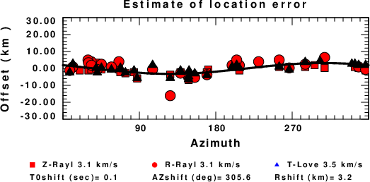
The derived shift in origin time and epicentral coordinates are given at the bottom of the figure.
Velocity Model
The WUS.model used for the waveform synthetic seismograms and for the surface wave eigenfunctions and dispersion is as follows
(The format is in the model96 format of Computer Programs in Seismology).
MODEL.01
Model after     8 iterations
ISOTROPIC
KGS
FLAT EARTH
1-D
CONSTANT VELOCITY
LINE08
LINE09
LINE10
LINE11
      H(KM)   VP(KM/S)   VS(KM/S) RHO(GM/CC)         QP         QS       ETAP       ETAS      FREFP      FREFS
     1.9000     3.4065     2.0089     2.2150  0.302E-02  0.679E-02   0.00       0.00       1.00       1.00
     6.1000     5.5445     3.2953     2.6089  0.349E-02  0.784E-02   0.00       0.00       1.00       1.00
    13.0000     6.2708     3.7396     2.7812  0.212E-02  0.476E-02   0.00       0.00       1.00       1.00
    19.0000     6.4075     3.7680     2.8223  0.111E-02  0.249E-02   0.00       0.00       1.00       1.00
     0.0000     7.9000     4.6200     3.2760  0.164E-10  0.370E-10   0.00       0.00       1.00       1.00
Last Changed Tue Apr 23 05:51:14 AM CDT 2024