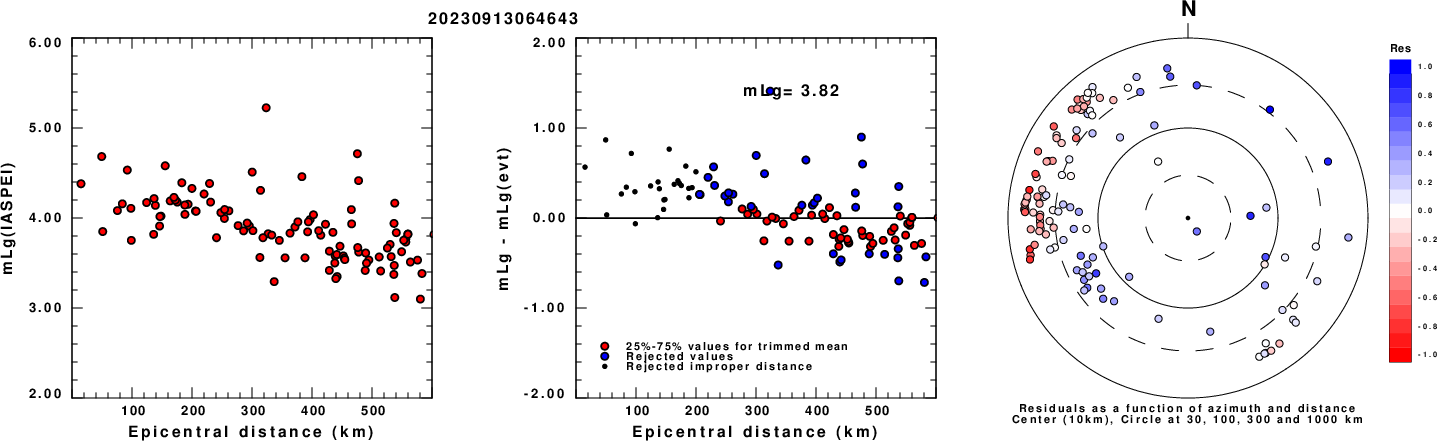
Left: mLg computed using the IASPEI formula. Center: mLg residuals versus epicentral distance ; the values used for the trimmed mean magnitude estimate are indicated. Right: residuals as a function of distance and azimuth.
The ANSS event ID is us7000kvgv and the event page is at https://earthquake.usgs.gov/earthquakes/eventpage/us7000kvgv/executive.
2023/09/13 06:46:43 61.352 -139.944 4.0 4 Yukon, Canada
 USGS/SLU Moment Tensor Solution
 ENS  2023/09/13 06:46:43:0  61.35 -139.94   4.0 4.0 Yukon, Canada

 Stations used:
   AK.BAE AK.BARK AK.BARN AK.BAT AK.BERG AK.BESE AK.BGLC
   AK.BMR AK.BRLK AK.CCB AK.CRQ AK.CUT AK.CYK AK.DHY AK.DIV
   AK.EYAK AK.FIRE AK.GHO AK.GLB AK.GLI AK.GRIN AK.H24K AK.HDA
   AK.HIN AK.I23K AK.I26K AK.I27K AK.ISLE AK.J25K AK.J26L
   AK.JIS AK.K24K AK.K27K AK.KHIT AK.KIAG AK.KLU AK.KNK
   AK.L22K AK.LOGN AK.M23K AK.M27K AK.MCAR AK.MCK AK.MDM
   AK.MESA AK.NEA2 AK.PAX AK.PNL AK.POKR AK.PS08 AK.PS09
   AK.PS10 AK.PS12 AK.PTPK AK.PWL AK.RC01 AK.RIDG AK.RND
   AK.S31K AK.S32K AK.SAMH AK.SAW AK.SCM AK.SCRK AK.TGL AK.VMT
   AK.VRDI AK.WAX AK.WRH AT.MENT AT.PMR AT.SIT AV.EDES AV.EDSO
   AV.N25K AV.WACK CN.ATLI CN.BRWY CN.BVCY CN.DAWY CN.HYT
   CN.PLBC CN.WHY CN.YUK3 CN.YUK4 CN.YUK6 CN.YUK7 CN.YUK8
   EO.KLRS IM.IL31 IU.COLA NY.MAYO US.EGAK

 Filtering commands used:
   cut o DIST/3.3 -40 o DIST/3.3 +50
   rtr
   taper w 0.1
   hp c 0.03 n 3
   lp c 0.08 n 3

 Best Fitting Double Couple
  Mo = 1.17e+22 dyne-cm
  Mw = 3.98
  Z  = 14 km
  Plane   Strike  Dip  Rake
   NP1      146    60   145
   NP2      255    60    35
  Principal Axes:
   Axis    Value   Plunge  Azimuth
    T   1.17e+22     45     110
    N   0.00e+00     45     291
    P  -1.17e+22      0     200

 Moment Tensor: (dyne-cm)
    Component   Value
       Mxx    -9.61e+21
       Mxy    -5.76e+21
       Mxz    -2.01e+21
       Myy     3.78e+21
       Myz     5.52e+21
       Mzz     5.84e+21


                     --------------
                 ----------------------
              ##--------------------------
             ###---------------------------
           #####-----------------------------
          ######------------------------------
         #######---------------#########-------
        #########------#######################--
        #########--#############################
       #########--###############################
       ######------##############################
       ####---------#############################
       ###-----------################   #########
        --------------############### T ########
        ---------------##############   ########
         ----------------######################
          -----------------###################
           ------------------################
             ------------------############
              ---------------------#######
                 ---   ----------------
                     P ------------


 Global CMT Convention Moment Tensor:
      R          T          P
  5.84e+21  -2.01e+21  -5.52e+21
 -2.01e+21  -9.61e+21   5.76e+21
 -5.52e+21   5.76e+21   3.78e+21


Details of the solution is found at

http://www.eas.slu.edu/eqc/eqc_mt/MECH.NA/20230913064643/index.html
|
      STK = 255
      DIP = 60
     RAKE = 35
       MW = 3.98
       HS = 14.0
The NDK file is 20230913064643.ndk The waveform inversion is preferred.
Given the availability of digital waveforms for determination of the moment tensor, this section documents the added processing leading to mLg, if appropriate to the region, and ML by application of the respective IASPEI formulae. As a research study, the linear distance term of the IASPEI formula for ML is adjusted to remove a linear distance trend in residuals to give a regionally defined ML. The defined ML uses horizontal component recordings, but the same procedure is applied to the vertical components since there may be some interest in vertical component ground motions. Residual plots versus distance may indicate interesting features of ground motion scaling in some distance ranges. A residual plot of the regionalized magnitude is given as a function of distance and azimuth, since data sets may transcend different wave propagation provinces.
Left: mLg computed using the IASPEI formula. Center: mLg residuals versus epicentral distance ; the values used for the trimmed mean magnitude estimate are indicated.
Right: residuals as a function of distance and azimuth.
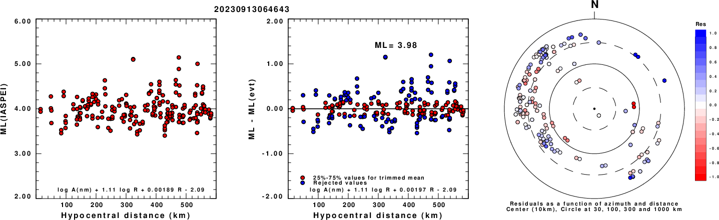
Left: ML computed using the IASPEI formula for Horizontal components. Center: ML residuals computed using a modified IASPEI formula that accounts for path specific attenuation; the values used for the trimmed mean are indicated. The ML relation used for each figure is given at the bottom of each plot.
Right: Residuals from new relation as a function of distance and azimuth.
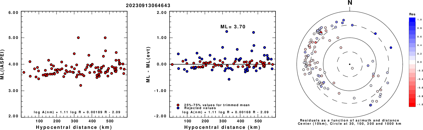
Left: ML computed using the IASPEI formula for Vertical components (research). Center: ML residuals computed using a modified IASPEI formula that accounts for path specific attenuation; the values used for the trimmed mean are indicated. The ML relation used for each figure is given at the bottom of each plot.
Right: Residuals from new relation as a function of distance and azimuth.
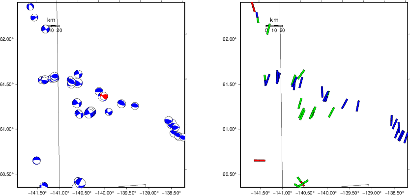 |
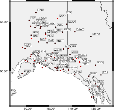
The focal mechanism was determined using broadband seismic waveforms. The location of the event (star) and the stations used for (red) the waveform inversion are shown in the next figure.
|
|
|
The program wvfgrd96 was used with good traces observed at short distance to determine the focal mechanism, depth and seismic moment. This technique requires a high quality signal and well determined velocity model for the Green's functions. To the extent that these are the quality data, this type of mechanism should be preferred over the radiation pattern technique which requires the separate step of defining the pressure and tension quadrants and the correct strike.
The observed and predicted traces are filtered using the following gsac commands:
cut o DIST/3.3 -40 o DIST/3.3 +50
rtr
taper w 0.1
hp c 0.03 n 3
lp c 0.08 n 3
The results of this grid search are as follow:
           DEPTH  STK   DIP  RAKE   MW    FIT
WVFGRD96    1.0   160    55    50   3.59 0.3211
WVFGRD96    2.0   170    50    60   3.71 0.3769
WVFGRD96    3.0   340    90    50   3.77 0.3988
WVFGRD96    4.0   155    85   -50   3.79 0.4463
WVFGRD96    5.0   150    80   -50   3.81 0.4844
WVFGRD96    6.0   150    75   -45   3.82 0.5130
WVFGRD96    7.0   145    70   -45   3.84 0.5334
WVFGRD96    8.0   140    65   -50   3.91 0.5410
WVFGRD96    9.0   135    60   -55   3.93 0.5508
WVFGRD96   10.0   135    60   -55   3.94 0.5514
WVFGRD96   11.0   260    55    45   3.95 0.5533
WVFGRD96   12.0   260    55    45   3.96 0.5634
WVFGRD96   13.0   260    60    45   3.98 0.5684
WVFGRD96   14.0   255    60    35   3.98 0.5710
WVFGRD96   15.0   255    60    35   3.99 0.5698
WVFGRD96   16.0   255    60    35   4.00 0.5656
WVFGRD96   17.0   255    60    35   4.01 0.5588
WVFGRD96   18.0   255    60    35   4.02 0.5498
WVFGRD96   19.0   255    60    35   4.03 0.5393
WVFGRD96   20.0   255    60    35   4.04 0.5279
WVFGRD96   21.0   255    60    35   4.05 0.5158
WVFGRD96   22.0   255    60    30   4.06 0.5026
WVFGRD96   23.0   255    60    30   4.07 0.4891
WVFGRD96   24.0   255    60    30   4.07 0.4758
WVFGRD96   25.0   255    60    30   4.08 0.4631
WVFGRD96   26.0   255    60    30   4.08 0.4503
WVFGRD96   27.0   255    60    30   4.09 0.4372
WVFGRD96   28.0   255    60    30   4.10 0.4240
WVFGRD96   29.0   255    60    30   4.10 0.4112
The best solution is
WVFGRD96 14.0 255 60 35 3.98 0.5710
The mechanism corresponding to the best fit is
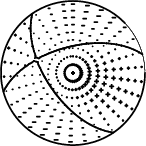
|
|
|
The best fit as a function of depth is given in the following figure:
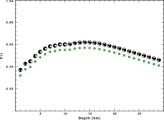
|
|
|
The comparison of the observed and predicted waveforms is given in the next figure. The red traces are the observed and the blue are the predicted. Each observed-predicted component is plotted to the same scale and peak amplitudes are indicated by the numbers to the left of each trace. A pair of numbers is given in black at the right of each predicted traces. The upper number it the time shift required for maximum correlation between the observed and predicted traces. This time shift is required because the synthetics are not computed at exactly the same distance as the observed, the velocity model used in the predictions may not be perfect and the epicentral parameters may be be off. A positive time shift indicates that the prediction is too fast and should be delayed to match the observed trace (shift to the right in this figure). A negative value indicates that the prediction is too slow. The lower number gives the percentage of variance reduction to characterize the individual goodness of fit (100% indicates a perfect fit).
The bandpass filter used in the processing and for the display was
cut o DIST/3.3 -40 o DIST/3.3 +50
rtr
taper w 0.1
hp c 0.03 n 3
lp c 0.08 n 3
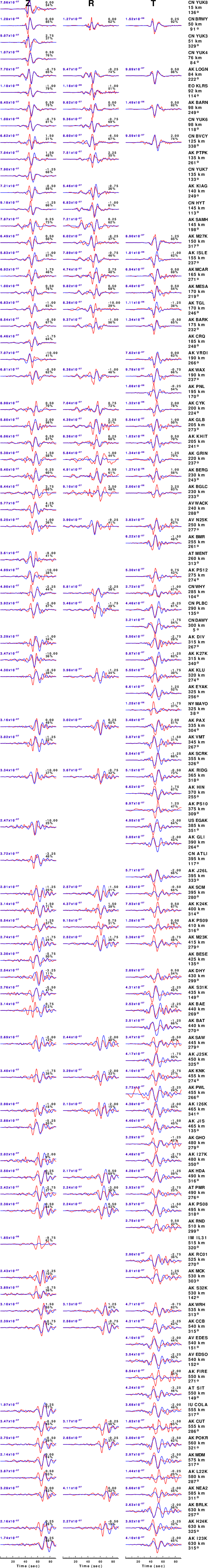
|
| Figure 3. Waveform comparison for selected depth. Red: observed; Blue - predicted. The time shift with respect to the model prediction is indicated. The percent of fit is also indicated. The time scale is relative to the first trace sample. |
|
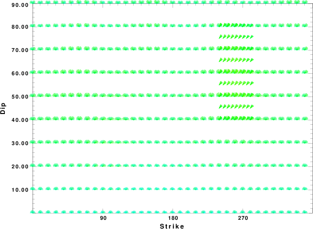
| Focal mechanism sensitivity at the preferred depth. The red color indicates a very good fit to the waveforms. Each solution is plotted as a vector at a given value of strike and dip with the angle of the vector representing the rake angle, measured, with respect to the upward vertical (N) in the figure. |
A check on the assumed source location is possible by looking at the time shifts between the observed and predicted traces. The time shifts for waveform matching arise for several reasons:
Time_shift = A + B cos Azimuth + C Sin Azimuth
The time shifts for this inversion lead to the next figure:
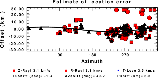
The derived shift in origin time and epicentral coordinates are given at the bottom of the figure.
The WUS.model used for the waveform synthetic seismograms and for the surface wave eigenfunctions and dispersion is as follows (The format is in the model96 format of Computer Programs in Seismology).
MODEL.01
Model after     8 iterations
ISOTROPIC
KGS
FLAT EARTH
1-D
CONSTANT VELOCITY
LINE08
LINE09
LINE10
LINE11
      H(KM)   VP(KM/S)   VS(KM/S) RHO(GM/CC)         QP         QS       ETAP       ETAS      FREFP      FREFS
     1.9000     3.4065     2.0089     2.2150  0.302E-02  0.679E-02   0.00       0.00       1.00       1.00
     6.1000     5.5445     3.2953     2.6089  0.349E-02  0.784E-02   0.00       0.00       1.00       1.00
    13.0000     6.2708     3.7396     2.7812  0.212E-02  0.476E-02   0.00       0.00       1.00       1.00
    19.0000     6.4075     3.7680     2.8223  0.111E-02  0.249E-02   0.00       0.00       1.00       1.00
     0.0000     7.9000     4.6200     3.2760  0.164E-10  0.370E-10   0.00       0.00       1.00       1.00