Location
Location ANSS
The ANSS event ID is ak0238x1rasm and the event page is at
https://earthquake.usgs.gov/earthquakes/eventpage/ak0238x1rasm/executive.
2023/07/13 12:59:58 62.987 -150.466 101.5 3.6 Alaska
Focal Mechanism
 USGS/SLU Moment Tensor Solution
 ENS  2023/07/13 12:59:58:0  62.99 -150.47 101.5 3.6 Alaska

 Stations used:
   AK.CAST AK.CCB AK.DHY AK.GHO AK.HDA AK.J19K AK.J20K AK.K20K
   AK.K24K AK.KNK AK.L20K AK.MCK AK.MLY AK.PAX AK.PPLA AK.RND
   AK.SAW AK.SCM AK.SKN AK.WAT6 AK.WRH AT.PMR AV.SPCP AV.STLK
   IM.IL31 IU.COLA

 Filtering commands used:
   cut o DIST/3.5 -40 o DIST/3.5 +50
   rtr
   taper w 0.1
   hp c 0.03 n 3
   lp c 0.10 n 3

 Best Fitting Double Couple
  Mo = 5.89e+21 dyne-cm
  Mw = 3.78
  Z  = 116 km
  Plane   Strike  Dip  Rake
   NP1        2    84   130
   NP2      100    40    10
  Principal Axes:
   Axis    Value   Plunge  Azimuth
    T   5.89e+21     38     307
    N   0.00e+00     39     177
    P  -5.89e+21     28      62

 Moment Tensor: (dyne-cm)
    Component   Value
       Mxx     2.98e+20
       Mxy    -3.67e+21
       Mxz     5.97e+20
       Myy    -1.31e+21
       Myz    -4.41e+21
       Mzz     1.01e+21


                     ########------
                 ############----------
              ###############-------------
             #################-------------
           ###################---------------
          ######   ###########----------------
         ####### T ###########----------   ----
        ########   ###########---------- P -----
        ######################----------   -----
       -######################-------------------
       -######################-------------------
       --#####################-------------------
       ---####################-------------------
        ----#################-------------------
        ------###############-----------------##
         -------#############---------------###
          ---------##########------------#####
           --------------####-------#########
             ---------------###############
              --------------##############
                 -----------###########
                     ------########


 Global CMT Convention Moment Tensor:
      R          T          P
  1.01e+21   5.97e+20   4.41e+21
  5.97e+20   2.98e+20   3.67e+21
  4.41e+21   3.67e+21  -1.31e+21


Details of the solution is found at

http://www.eas.slu.edu/eqc/eqc_mt/MECH.NA/20230713125958/index.html
|
Preferred Solution
The preferred solution from an analysis of the surface-wave spectral amplitude radiation pattern, waveform inversion or first motion observations is
      STK = 100
      DIP = 40
     RAKE = 10
       MW = 3.78
       HS = 116.0
The NDK file is 20230713125958.ndk
The waveform inversion is preferred.
Magnitudes
Given the availability of digital waveforms for determination of the moment tensor, this section documents the added processing leading to mLg, if appropriate to the region, and ML by application of the respective IASPEI formulae. As a research study, the linear distance term of the IASPEI formula
for ML is adjusted to remove a linear distance trend in residuals to give a regionally defined ML. The defined ML uses horizontal component recordings, but the same procedure is applied to the vertical components since there may be some interest in vertical component ground motions. Residual plots versus distance may indicate interesting features of ground motion scaling in some distance ranges. A residual plot of the regionalized magnitude is given as a function of distance and azimuth, since data sets may transcend different wave propagation provinces.
ML Magnitude
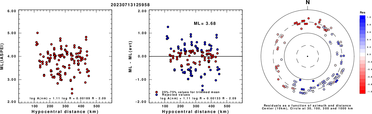
Left: ML computed using the IASPEI formula for Horizontal components. Center: ML residuals computed using a modified IASPEI formula that accounts for path specific attenuation; the values used for the trimmed mean are indicated. The ML relation used for each figure is given at the bottom of each plot.
Right: Residuals from new relation as a function of distance and azimuth.
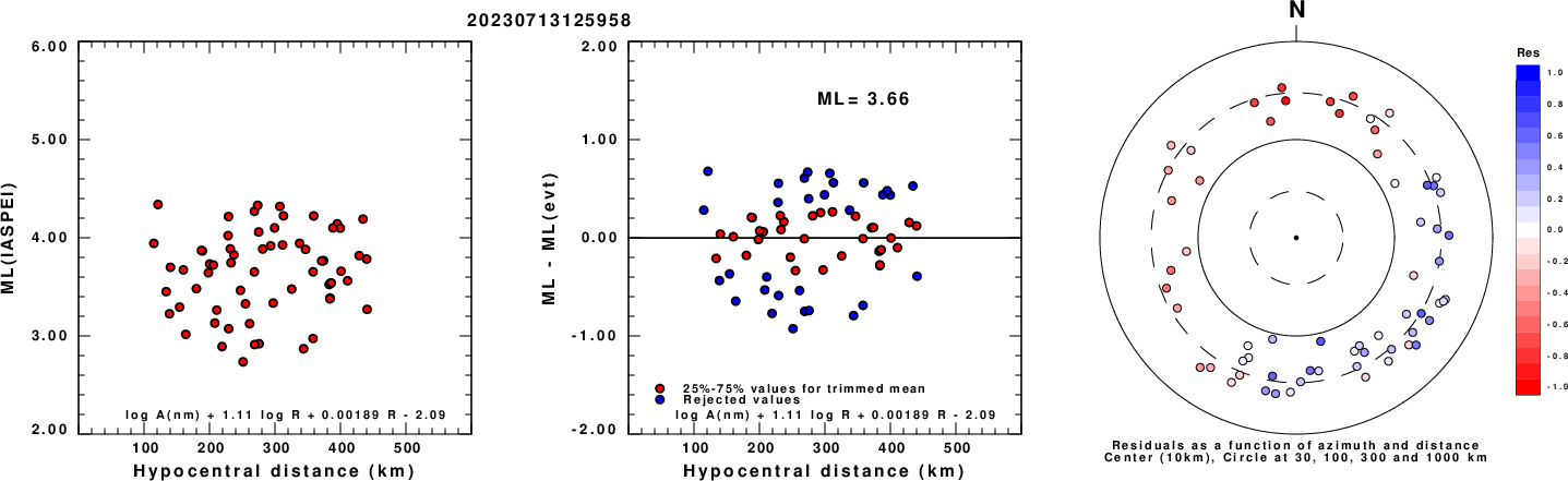
Left: ML computed using the IASPEI formula for Vertical components (research). Center: ML residuals computed using a modified IASPEI formula that accounts for path specific attenuation; the values used for the trimmed mean are indicated. The ML relation used for each figure is given at the bottom of each plot.
Right: Residuals from new relation as a function of distance and azimuth.
Context
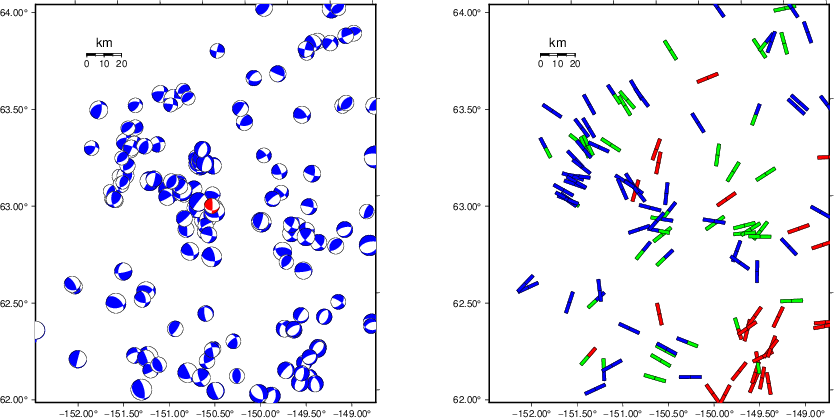
The left panel of the next figure presents the focal mechanism for this earthquake (red) in the context of other nearby events (blue) in the SLU Moment Tensor Catalog. The right panel shows the inferred direction of maximum compressive stress and the type of faulting (green is strike-slip, red is normal, blue is thrust; oblique is shown by a combination of colors). Thus context plot is useful for assessing the appropriateness of the moment tensor of this event.
Waveform Inversion using wvfgrd96
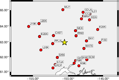
The focal mechanism was determined using broadband seismic waveforms. The location of the event (star) and the
stations used for (red) the waveform inversion are shown in the next figure.
|
|
Location of broadband stations used for waveform inversion
|
The program wvfgrd96 was used with good traces observed at short distance to determine the focal mechanism, depth and seismic moment. This technique requires a high quality signal and well determined velocity model for the Green's functions. To the extent that these are the quality data, this type of mechanism should be preferred over the radiation pattern technique which requires the separate step of defining the pressure and tension quadrants and the correct strike.
The observed and predicted traces are filtered using the following gsac commands:
cut o DIST/3.5 -40 o DIST/3.5 +50
rtr
taper w 0.1
hp c 0.03 n 3
lp c 0.10 n 3
The results of this grid search are as follow:
           DEPTH  STK   DIP  RAKE   MW    FIT
WVFGRD96    2.0   175    50   -70   2.86 0.1871
WVFGRD96    4.0    25    45     0   2.89 0.1946
WVFGRD96    6.0   210    55    25   2.95 0.2301
WVFGRD96    8.0   210    55    25   3.04 0.2522
WVFGRD96   10.0    30    60    20   3.08 0.2639
WVFGRD96   12.0    25    60    15   3.12 0.2690
WVFGRD96   14.0    25    60    15   3.15 0.2690
WVFGRD96   16.0    30    55    15   3.18 0.2631
WVFGRD96   18.0   130    75    40   3.19 0.2548
WVFGRD96   20.0   130    80    40   3.21 0.2541
WVFGRD96   22.0   300    75    30   3.26 0.2628
WVFGRD96   24.0   300    75    25   3.28 0.2719
WVFGRD96   26.0   295    80    25   3.31 0.2793
WVFGRD96   28.0   275    60     5   3.33 0.2881
WVFGRD96   30.0   275    65     0   3.35 0.2937
WVFGRD96   32.0   275    70     5   3.36 0.2954
WVFGRD96   34.0   275    70     5   3.37 0.2967
WVFGRD96   36.0   275    70     5   3.39 0.2922
WVFGRD96   38.0   100    75    20   3.42 0.2858
WVFGRD96   40.0   100    70    25   3.48 0.2896
WVFGRD96   42.0   100    70    25   3.51 0.2950
WVFGRD96   44.0   100    70    25   3.53 0.2962
WVFGRD96   46.0   100    70    25   3.55 0.2975
WVFGRD96   48.0   100    75    25   3.57 0.3023
WVFGRD96   50.0   100    80    30   3.59 0.3107
WVFGRD96   52.0   100    80    30   3.61 0.3191
WVFGRD96   54.0   105    75    40   3.64 0.3287
WVFGRD96   56.0   105    75    40   3.65 0.3376
WVFGRD96   58.0   105    55    20   3.63 0.3500
WVFGRD96   60.0   105    55    20   3.64 0.3640
WVFGRD96   62.0   105    55    20   3.65 0.3775
WVFGRD96   64.0   105    50    20   3.65 0.3933
WVFGRD96   66.0   105    55    20   3.66 0.4074
WVFGRD96   68.0   105    55    20   3.67 0.4204
WVFGRD96   70.0   105    50    20   3.68 0.4325
WVFGRD96   72.0   100    45    15   3.68 0.4455
WVFGRD96   74.0   100    45    15   3.69 0.4570
WVFGRD96   76.0    95    45    10   3.69 0.4691
WVFGRD96   78.0   100    40    15   3.70 0.4800
WVFGRD96   80.0   100    40    15   3.71 0.4893
WVFGRD96   82.0   100    45    15   3.71 0.4992
WVFGRD96   84.0   100    45    15   3.71 0.5101
WVFGRD96   86.0   100    45    15   3.72 0.5198
WVFGRD96   88.0   100    40    15   3.73 0.5294
WVFGRD96   90.0   100    40    15   3.73 0.5392
WVFGRD96   92.0   100    40    15   3.73 0.5489
WVFGRD96   94.0   100    40    15   3.74 0.5583
WVFGRD96   96.0   100    40    15   3.74 0.5659
WVFGRD96   98.0   100    40    15   3.75 0.5726
WVFGRD96  100.0   100    40    15   3.75 0.5791
WVFGRD96  102.0   100    40    15   3.75 0.5843
WVFGRD96  104.0   100    40    10   3.76 0.5888
WVFGRD96  106.0   100    40    10   3.76 0.5933
WVFGRD96  108.0   100    40    10   3.77 0.5969
WVFGRD96  110.0   100    40    10   3.77 0.5989
WVFGRD96  112.0   100    40    10   3.77 0.6001
WVFGRD96  114.0   100    40    10   3.77 0.6011
WVFGRD96  116.0   100    40    10   3.78 0.6021
WVFGRD96  118.0   100    40    10   3.78 0.6013
WVFGRD96  120.0   100    40    10   3.78 0.5989
WVFGRD96  122.0   100    40    10   3.78 0.5966
WVFGRD96  124.0   100    40    10   3.78 0.5938
WVFGRD96  126.0   100    40    10   3.78 0.5916
WVFGRD96  128.0    95    45    10   3.78 0.5893
WVFGRD96  130.0   100    40    15   3.78 0.5868
WVFGRD96  132.0   100    40    15   3.78 0.5833
WVFGRD96  134.0   100    40    15   3.78 0.5796
WVFGRD96  136.0   100    40    15   3.78 0.5761
WVFGRD96  138.0   100    45    15   3.78 0.5734
WVFGRD96  140.0   100    45    15   3.78 0.5708
WVFGRD96  142.0    95    50     5   3.79 0.5671
WVFGRD96  144.0   100    45    15   3.79 0.5631
WVFGRD96  146.0    95    55     5   3.79 0.5612
WVFGRD96  148.0    95    55     5   3.80 0.5592
WVFGRD96  150.0    95    55     5   3.80 0.5569
WVFGRD96  152.0    95    55     5   3.80 0.5532
WVFGRD96  154.0    95    55     5   3.80 0.5517
WVFGRD96  156.0    95    55     5   3.80 0.5498
WVFGRD96  158.0    95    55     5   3.81 0.5467
The best solution is
WVFGRD96 116.0 100 40 10 3.78 0.6021
The mechanism corresponding to the best fit is
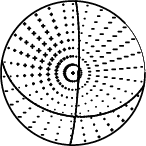
|
|
Figure 1. Waveform inversion focal mechanism
|
The best fit as a function of depth is given in the following figure:
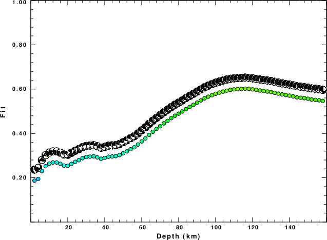
|
|
Figure 2. Depth sensitivity for waveform mechanism
|
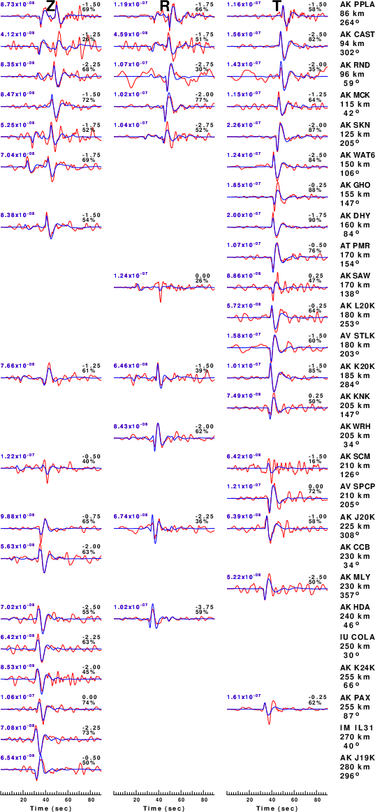
The comparison of the observed and predicted waveforms is given in the next figure. The red traces are the observed and the blue are the predicted.
Each observed-predicted component is plotted to the same scale and peak amplitudes are indicated by the numbers to the left of each trace. A pair of numbers is given in black at the right of each predicted traces. The upper number it the time shift required for maximum correlation between the observed and predicted traces. This time shift is required because the synthetics are not computed at exactly the same distance as the observed, the velocity model used in the predictions may not be perfect and the epicentral parameters may be be off.
A positive time shift indicates that the prediction is too fast and should be delayed to match the observed trace (shift to the right in this figure). A negative value indicates that the prediction is too slow. The lower number gives the percentage of variance reduction to characterize the individual goodness of fit (100% indicates a perfect fit).
The bandpass filter used in the processing and for the display was
cut o DIST/3.5 -40 o DIST/3.5 +50
rtr
taper w 0.1
hp c 0.03 n 3
lp c 0.10 n 3
|
|
Figure 3. Waveform comparison for selected depth. Red: observed; Blue - predicted. The time shift with respect to the model prediction is indicated. The percent of fit is also indicated. The time scale is relative to the first trace sample.
|
|
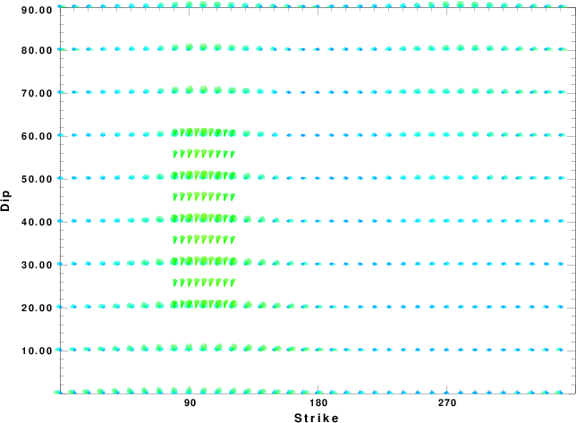
|
Focal mechanism sensitivity at the preferred depth. The red color indicates a very good fit to the waveforms.
Each solution is plotted as a vector at a given value of strike and dip with the angle of the vector representing the rake angle, measured, with respect to the upward vertical (N) in the figure.
|
A check on the assumed source location is possible by looking at the time shifts between the observed and predicted traces. The time shifts for waveform matching arise for several reasons:
- The origin time and epicentral distance are incorrect
- The velocity model used for the inversion is incorrect
- The velocity model used to define the P-arrival time is not the
same as the velocity model used for the waveform inversion
(assuming that the initial trace alignment is based on the
P arrival time)
Assuming only a mislocation, the time shifts are fit to a functional form:
Time_shift = A + B cos Azimuth + C Sin Azimuth
The time shifts for this inversion lead to the next figure:
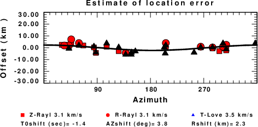
The derived shift in origin time and epicentral coordinates are given at the bottom of the figure.
Velocity Model
The WUS.model used for the waveform synthetic seismograms and for the surface wave eigenfunctions and dispersion is as follows
(The format is in the model96 format of Computer Programs in Seismology).
MODEL.01
Model after     8 iterations
ISOTROPIC
KGS
FLAT EARTH
1-D
CONSTANT VELOCITY
LINE08
LINE09
LINE10
LINE11
      H(KM)   VP(KM/S)   VS(KM/S) RHO(GM/CC)         QP         QS       ETAP       ETAS      FREFP      FREFS
     1.9000     3.4065     2.0089     2.2150  0.302E-02  0.679E-02   0.00       0.00       1.00       1.00
     6.1000     5.5445     3.2953     2.6089  0.349E-02  0.784E-02   0.00       0.00       1.00       1.00
    13.0000     6.2708     3.7396     2.7812  0.212E-02  0.476E-02   0.00       0.00       1.00       1.00
    19.0000     6.4075     3.7680     2.8223  0.111E-02  0.249E-02   0.00       0.00       1.00       1.00
     0.0000     7.9000     4.6200     3.2760  0.164E-10  0.370E-10   0.00       0.00       1.00       1.00
Last Changed Tue Apr 23 01:19:57 AM CDT 2024