Location

Location ANSS

The ANSS event ID is ci40230055 and the event page is at https://earthquake.usgs.gov/earthquakes/eventpage/ci40230055/executive.

2023/05/21 03:26:29 37.284 -117.584 5.3 4.26 California

Focal Mechanism

USGS/SLU Moment Tensor Solution ENS 2023/05/21 03:26:29:0 37.28 -117.58 5.3 4.3 California Stations used: AE.W13A BK.HELL BK.MMI BK.OVRO BK.WELL BK.WINE BK.YUBA CI.BCW CI.BEL CI.BFS CI.CCC CI.CSH CI.CTW CI.DAN CI.DSC CI.DTP CI.ELS2 CI.FUR CI.GRA CI.GSC CI.HHL CI.IRM CI.ISA CI.LRL CI.LUC2 CI.MSC CI.MTP CI.NEE2 CI.OSI CI.PALA CI.PASC CI.RAG CI.SBB2 CI.SHO CI.TEH CI.TPO CI.WGR GS.MCA04 II.PFO IM.NV31 NN.BEK NN.DIX NN.GMN NN.GWY NN.KVN NN.LHV NN.MPK NN.PNT NN.PRN NN.PYM2 NN.Q09A NN.REDF NN.SHP NN.UNVG SN.TPW US.ELK US.TPNV UU.CCUT UU.FOR1 UU.PSUT UU.SZCU UU.VRUT Filtering commands used: cut o DIST/3.3 -40 o DIST/3.3 +50 rtr taper w 0.1 hp c 0.03 n 3 lp c 0.07 n 3 Best Fitting Double Couple Mo = 2.34e+22 dyne-cm Mw = 4.18 Z = 8 km Plane Strike Dip Rake NP1 199 46 -80 NP2 5 45 -100 Principal Axes: Axis Value Plunge Azimuth T 2.34e+22 0 282 N 0.00e+00 7 12 P -2.34e+22 83 189 Moment Tensor: (dyne-cm) Component Value Mxx 6.75e+20 Mxy -4.84e+21 Mxz 2.87e+21 Myy 2.24e+22 Myz 2.51e+20 Mzz -2.31e+22 ###########--# ############-----##### ############---------####### ###########------------####### ###########---------------######## ###########-----------------######## ###########------------------######### ###########--------------------######### #########---------------------######### T ########----------------------########## ########----------------------########## #########---------- ----------########## #########---------- P ----------########## ########---------- ----------######### ########----------------------########## #######----------------------######### ######---------------------######### ######-------------------######### #####-----------------######## ####---------------######### ###-----------######## --------###### Global CMT Convention Moment Tensor: R T P -2.31e+22 2.87e+21 -2.51e+20 2.87e+21 6.75e+20 4.84e+21 -2.51e+20 4.84e+21 2.24e+22 Details of the solution is found at http://www.eas.slu.edu/eqc/eqc_mt/MECH.NA/20230521032629/index.html

Preferred Solution

      STK = 5
      DIP = 45
     RAKE = -100
       MW = 4.18
       HS = 8.0

The NDK file is 20230521032629.ndk The waveform inversion is preferred.

Moment Tensor Comparison

The following compares this source inversion to those provided by others. The purpose is to look for major differences and also to note slight differences that might be inherent to the processing procedure. For completeness the USGS/SLU solution is repeated from above.

SLU	CI	NC
USGS/SLU Moment Tensor Solution ENS 2023/05/21 03:26:29:0 37.28 -117.58 5.3 4.3 California Stations used: AE.W13A BK.HELL BK.MMI BK.OVRO BK.WELL BK.WINE BK.YUBA CI.BCW CI.BEL CI.BFS CI.CCC CI.CSH CI.CTW CI.DAN CI.DSC CI.DTP CI.ELS2 CI.FUR CI.GRA CI.GSC CI.HHL CI.IRM CI.ISA CI.LRL CI.LUC2 CI.MSC CI.MTP CI.NEE2 CI.OSI CI.PALA CI.PASC CI.RAG CI.SBB2 CI.SHO CI.TEH CI.TPO CI.WGR GS.MCA04 II.PFO IM.NV31 NN.BEK NN.DIX NN.GMN NN.GWY NN.KVN NN.LHV NN.MPK NN.PNT NN.PRN NN.PYM2 NN.Q09A NN.REDF NN.SHP NN.UNVG SN.TPW US.ELK US.TPNV UU.CCUT UU.FOR1 UU.PSUT UU.SZCU UU.VRUT Filtering commands used: cut o DIST/3.3 -40 o DIST/3.3 +50 rtr taper w 0.1 hp c 0.03 n 3 lp c 0.07 n 3 Best Fitting Double Couple Mo = 2.34e+22 dyne-cm Mw = 4.18 Z = 8 km Plane Strike Dip Rake NP1 199 46 -80 NP2 5 45 -100 Principal Axes: Axis Value Plunge Azimuth T 2.34e+22 0 282 N 0.00e+00 7 12 P -2.34e+22 83 189 Moment Tensor: (dyne-cm) Component Value Mxx 6.75e+20 Mxy -4.84e+21 Mxz 2.87e+21 Myy 2.24e+22 Myz 2.51e+20 Mzz -2.31e+22 ###########--# ############-----##### ############---------####### ###########------------####### ###########---------------######## ###########-----------------######## ###########------------------######### ###########--------------------######### #########---------------------######### T ########----------------------########## ########----------------------########## #########---------- ----------########## #########---------- P ----------########## ########---------- ----------######### ########----------------------########## #######----------------------######### ######---------------------######### ######-------------------######### #####-----------------######## ####---------------######### ###-----------######## --------###### Global CMT Convention Moment Tensor: R T P -2.31e+22 2.87e+21 -2.51e+20 2.87e+21 6.75e+20 4.84e+21 -2.51e+20 4.84e+21 2.24e+22 Details of the solution is found at http://www.eas.slu.edu/eqc/eqc_mt/MECH.NA/20230521032629/index.html	Moment Tensor (TMTS) Moment 3.044e+15 N-m Magnitude 4.26 Depth 8.0 km Percent DC 92% Half Duration - Catalog CI Data Source CI 2 Contributor CI 2 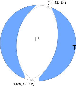Nodal Planes Plane Strike Dip Rake NP1 14 48 -84 NP2 185 42 -96 Principal Axes Axis Value Plunge Azimuth T 3.105e+15 N-m 3 100 N -0.127e+15 N-m 4 190 P -2.978e+15 N-m 85 335	ontributed by NC 3 last updated 2023-05-21 07:11:42 (UTC) The data below are the most preferred data available The data below have NOT been reviewed by a scientist. 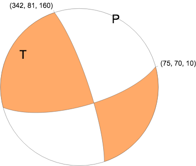Catalog NC Data Source NC 3 Contributor NC 3 Nodal Planes Plane Strike Dip Rake NP1 342 81 160 NP2 75 70 10

Magnitudes

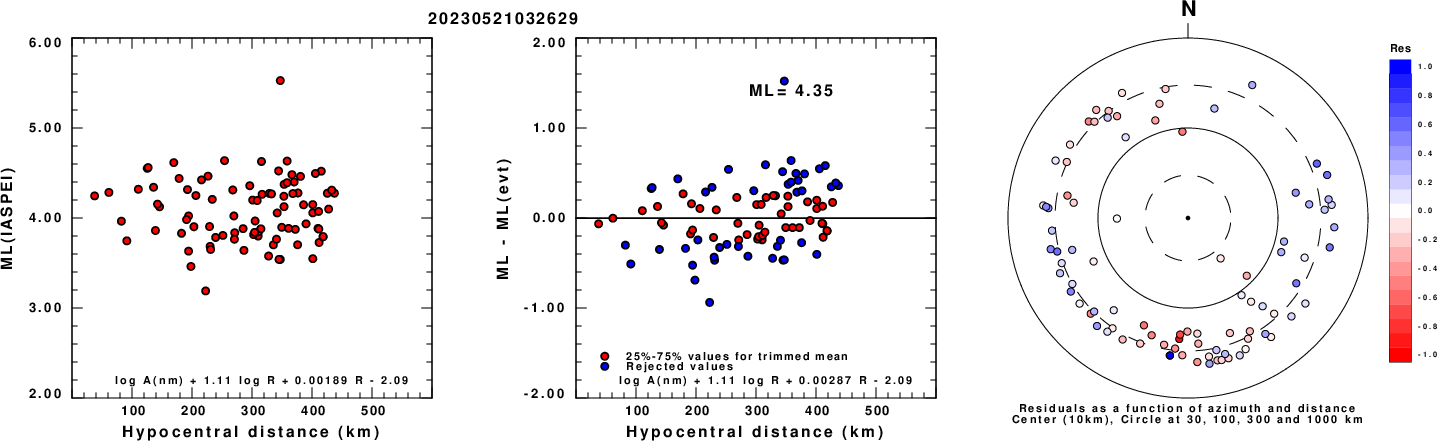
Given the availability of digital waveforms for determination of the moment tensor, this section documents the added processing leading to mLg, if appropriate to the region, and M_L by application of the respective IASPEI formulae. As a research study, the linear distance term of the IASPEI formula for M_L is adjusted to remove a linear distance trend in residuals to give a regionally defined M_L. The defined M_L uses horizontal component recordings, but the same procedure is applied to the vertical components since there may be some interest in vertical component ground motions. Residual plots versus distance may indicate interesting features of ground motion scaling in some distance ranges. A residual plot of the regionalized magnitude is given as a function of distance and azimuth, since data sets may transcend different wave propagation provinces.

ML Magnitude

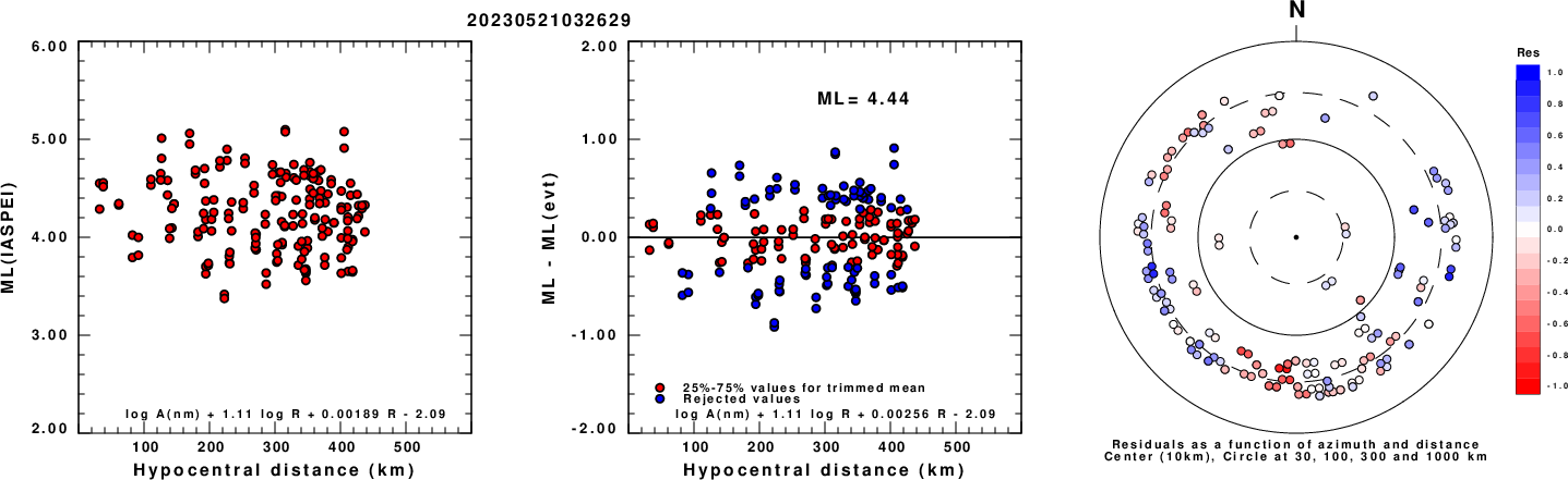
Left: ML computed using the IASPEI formula for Horizontal components. Center: ML residuals computed using a modified IASPEI formula that accounts for path specific attenuation; the values used for the trimmed mean are indicated. The ML relation used for each figure is given at the bottom of each plot. Right: Residuals from new relation as a function of distance and azimuth.

Left: ML computed using the IASPEI formula for Vertical components (research). Center: ML residuals computed using a modified IASPEI formula that accounts for path specific attenuation; the values used for the trimmed mean are indicated. The ML relation used for each figure is given at the bottom of each plot. Right: Residuals from new relation as a function of distance and azimuth.

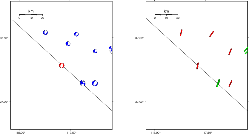
Context

Waveform Inversion using wvfgrd96

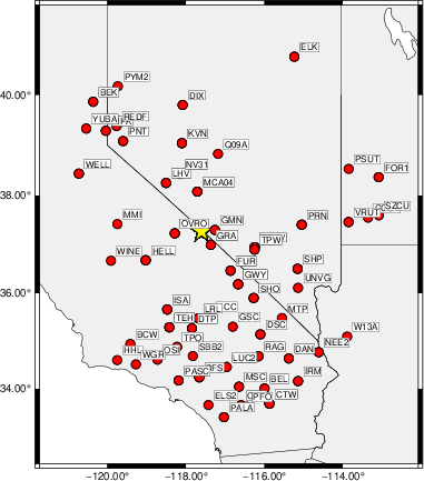
The focal mechanism was determined using broadband seismic waveforms. The location of the event (star) and the stations used for (red) the waveform inversion are shown in the next figure.

Location of broadband stations used for waveform inversion

The program wvfgrd96 was used with good traces observed at short distance to determine the focal mechanism, depth and seismic moment. This technique requires a high quality signal and well determined velocity model for the Green's functions. To the extent that these are the quality data, this type of mechanism should be preferred over the radiation pattern technique which requires the separate step of defining the pressure and tension quadrants and the correct strike.

The observed and predicted traces are filtered using the following gsac commands:

cut o DIST/3.3 -40 o DIST/3.3 +50
rtr
taper w 0.1
hp c 0.03 n 3 
lp c 0.07 n 3 

           DEPTH  STK   DIP  RAKE   MW    FIT
WVFGRD96    1.0    55    75   -25   3.77 0.3498
WVFGRD96    2.0   235    85   -40   3.92 0.4162
WVFGRD96    3.0   235    85   -50   3.99 0.4576
WVFGRD96    4.0   225    65   -45   4.01 0.5008
WVFGRD96    5.0   215    50   -60   4.07 0.5563
WVFGRD96    6.0   220    50   -50   4.08 0.5809
WVFGRD96    7.0   220    50   -50   4.09 0.5808
WVFGRD96    8.0     5    45  -100   4.18 0.6036
WVFGRD96    9.0   220    50   -50   4.14 0.5764
WVFGRD96   10.0   225    55   -40   4.13 0.5498
WVFGRD96   11.0   230    60   -30   4.12 0.5283
WVFGRD96   12.0   235    70   -20   4.12 0.5110
WVFGRD96   13.0   235    75   -20   4.12 0.4939
WVFGRD96   14.0   235    75   -15   4.13 0.4785
WVFGRD96   15.0   235    80   -15   4.14 0.4634
WVFGRD96   16.0   235    80   -15   4.15 0.4484
WVFGRD96   17.0   235    80   -15   4.15 0.4340
WVFGRD96   18.0   235    80   -15   4.16 0.4205
WVFGRD96   19.0   240    85   -10   4.16 0.4088
WVFGRD96   20.0   240    85   -10   4.16 0.3986
WVFGRD96   21.0   240    85   -10   4.17 0.3887
WVFGRD96   22.0   240    80   -10   4.18 0.3792
WVFGRD96   23.0   240    80   -10   4.18 0.3711
WVFGRD96   24.0   240    80   -10   4.19 0.3634
WVFGRD96   25.0   240    85   -10   4.19 0.3564
WVFGRD96   26.0   240    85   -10   4.20 0.3501
WVFGRD96   27.0    60    90    10   4.20 0.3444
WVFGRD96   28.0    60    80    10   4.21 0.3389
WVFGRD96   29.0    60    80    10   4.22 0.3341

The best solution is

WVFGRD96    8.0     5    45  -100   4.18 0.6036

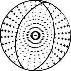
The mechanism corresponding to the best fit is

Figure 1. Waveform inversion focal mechanism

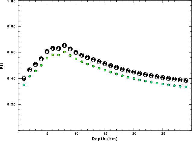
The best fit as a function of depth is given in the following figure:

Figure 2. Depth sensitivity for waveform mechanism

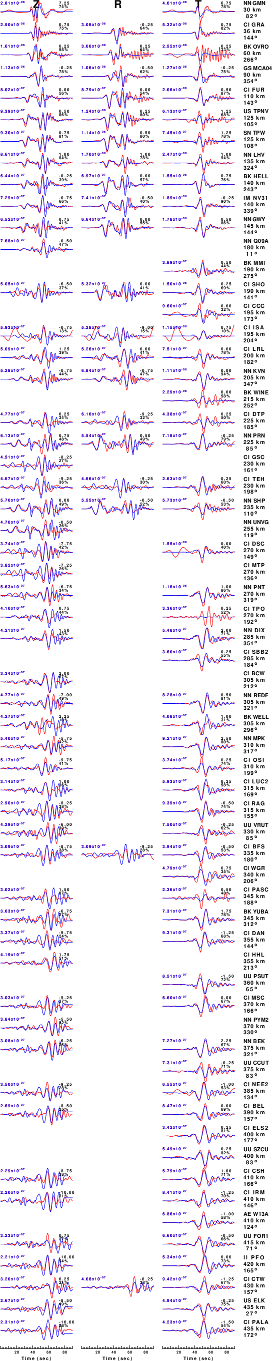
The comparison of the observed and predicted waveforms is given in the next figure. The red traces are the observed and the blue are the predicted. Each observed-predicted component is plotted to the same scale and peak amplitudes are indicated by the numbers to the left of each trace. A pair of numbers is given in black at the right of each predicted traces. The upper number it the time shift required for maximum correlation between the observed and predicted traces. This time shift is required because the synthetics are not computed at exactly the same distance as the observed, the velocity model used in the predictions may not be perfect and the epicentral parameters may be be off. A positive time shift indicates that the prediction is too fast and should be delayed to match the observed trace (shift to the right in this figure). A negative value indicates that the prediction is too slow. The lower number gives the percentage of variance reduction to characterize the individual goodness of fit (100% indicates a perfect fit).

The bandpass filter used in the processing and for the display was

cut o DIST/3.3 -40 o DIST/3.3 +50
rtr
taper w 0.1
hp c 0.03 n 3 
lp c 0.07 n 3 

Figure 3. Waveform comparison for selected depth. Red: observed; Blue - predicted. The time shift with respect to the model prediction is indicated. The percent of fit is also indicated. The time scale is relative to the first trace sample.

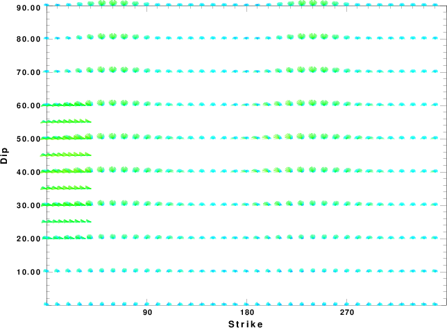
Focal mechanism sensitivity at the preferred depth. The red color indicates a very good fit to the waveforms. Each solution is plotted as a vector at a given value of strike and dip with the angle of the vector representing the rake angle, measured, with respect to the upward vertical (N) in the figure.

A check on the assumed source location is possible by looking at the time shifts between the observed and predicted traces. The time shifts for waveform matching arise for several reasons:

• The origin time and epicentral distance are incorrect
• The velocity model used for the inversion is incorrect
• The velocity model used to define the P-arrival time is not the same as the velocity model used for the waveform inversion (assuming that the initial trace alignment is based on the P arrival time)

 Time_shift = A + B cos Azimuth + C Sin Azimuth

The time shifts for this inversion lead to the next figure:

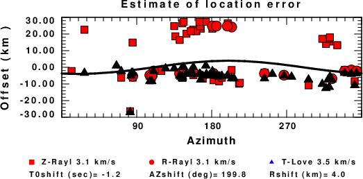
The derived shift in origin time and epicentral coordinates are given at the bottom of the figure.

Velocity Model

The WUS.model used for the waveform synthetic seismograms and for the surface wave eigenfunctions and dispersion is as follows (The format is in the model96 format of Computer Programs in Seismology).

MODEL.01
Model after     8 iterations
ISOTROPIC
KGS
FLAT EARTH
1-D
CONSTANT VELOCITY
LINE08
LINE09
LINE10
LINE11
      H(KM)   VP(KM/S)   VS(KM/S) RHO(GM/CC)         QP         QS       ETAP       ETAS      FREFP      FREFS
     1.9000     3.4065     2.0089     2.2150  0.302E-02  0.679E-02   0.00       0.00       1.00       1.00    
     6.1000     5.5445     3.2953     2.6089  0.349E-02  0.784E-02   0.00       0.00       1.00       1.00    
    13.0000     6.2708     3.7396     2.7812  0.212E-02  0.476E-02   0.00       0.00       1.00       1.00    
    19.0000     6.4075     3.7680     2.8223  0.111E-02  0.249E-02   0.00       0.00       1.00       1.00    
     0.0000     7.9000     4.6200     3.2760  0.164E-10  0.370E-10   0.00       0.00       1.00       1.00