Location
Location ANSS
The ANSS event ID is ak022fwcrh7q and the event page is at
https://earthquake.usgs.gov/earthquakes/eventpage/ak022fwcrh7q/executive.
2022/12/12 08:09:01 59.278 -150.643 36.7 4.7 Alaska
Focal Mechanism
 USGS/SLU Moment Tensor Solution
 ENS  2022/12/12 08:09:01:0  59.28 -150.64  36.7 4.7 Alaska

 Stations used:
   AK.BRLK AK.CNP AK.DIV AK.FID AK.GHO AK.GLI AK.HOM AK.KLU
   AK.KNK AK.N19K AK.O18K AK.O19K AK.Q19K AK.SAW AK.SLK AK.SWD
   AV.ACH AV.ILS AV.RED

 Filtering commands used:
   cut o DIST/3.3 -40 o DIST/3.3 +50
   rtr
   taper w 0.1
   hp c 0.03 n 3
   lp c 0.08 n 3

 Best Fitting Double Couple
  Mo = 1.07e+23 dyne-cm
  Mw = 4.62
  Z  = 44 km
  Plane   Strike  Dip  Rake
   NP1      225    60   -45
   NP2      342    52   -141
  Principal Axes:
   Axis    Value   Plunge  Azimuth
    T   1.07e+23      5     285
    N   0.00e+00     38      18
    P  -1.07e+23     52     189

 Moment Tensor: (dyne-cm)
    Component   Value
       Mxx    -3.28e+22
       Mxy    -3.28e+22
       Mxz     5.36e+22
       Myy     9.84e+22
       Myz    -7.98e+15
       Mzz    -6.56e+22


                     #-------------
                 #########-------------
              ###############-------------
             ##################-----#######
           ##################################
          ##################------############
         #################---------############
          ##############------------############
        T ############--------------############
          ##########-----------------############
       ############-------------------###########
       ###########--------------------###########
       #########----------------------###########
        #######------------------------#########
        #######------------------------#########
         #####-----------   -----------########
          ####----------- P ----------########
           ##------------   ----------#######
             -------------------------#####
              -----------------------#####
                 -------------------###
                     --------------


 Global CMT Convention Moment Tensor:
      R          T          P
 -6.56e+22   5.36e+22   7.98e+15
  5.36e+22  -3.28e+22   3.28e+22
  7.98e+15   3.28e+22   9.84e+22


Details of the solution is found at

http://www.eas.slu.edu/eqc/eqc_mt/MECH.NA/20221212080901/index.html
|
Preferred Solution
The preferred solution from an analysis of the surface-wave spectral amplitude radiation pattern, waveform inversion or first motion observations is
      STK = 225
      DIP = 60
     RAKE = -45
       MW = 4.62
       HS = 44.0
The NDK file is 20221212080901.ndk
The waveform inversion is preferred.
Moment Tensor Comparison
The following compares this source inversion to those provided by others. The purpose is to look for major differences and also to note slight differences that might be inherent to the processing procedure. For completeness the USGS/SLU solution is repeated from above.
| SLU |
USGSMWR |
 USGS/SLU Moment Tensor Solution
 ENS  2022/12/12 08:09:01:0  59.28 -150.64  36.7 4.7 Alaska

 Stations used:
   AK.BRLK AK.CNP AK.DIV AK.FID AK.GHO AK.GLI AK.HOM AK.KLU
   AK.KNK AK.N19K AK.O18K AK.O19K AK.Q19K AK.SAW AK.SLK AK.SWD
   AV.ACH AV.ILS AV.RED

 Filtering commands used:
   cut o DIST/3.3 -40 o DIST/3.3 +50
   rtr
   taper w 0.1
   hp c 0.03 n 3
   lp c 0.08 n 3

 Best Fitting Double Couple
  Mo = 1.07e+23 dyne-cm
  Mw = 4.62
  Z  = 44 km
  Plane   Strike  Dip  Rake
   NP1      225    60   -45
   NP2      342    52   -141
  Principal Axes:
   Axis    Value   Plunge  Azimuth
    T   1.07e+23      5     285
    N   0.00e+00     38      18
    P  -1.07e+23     52     189

 Moment Tensor: (dyne-cm)
    Component   Value
       Mxx    -3.28e+22
       Mxy    -3.28e+22
       Mxz     5.36e+22
       Myy     9.84e+22
       Myz    -7.98e+15
       Mzz    -6.56e+22


                     #-------------
                 #########-------------
              ###############-------------
             ##################-----#######
           ##################################
          ##################------############
         #################---------############
          ##############------------############
        T ############--------------############
          ##########-----------------############
       ############-------------------###########
       ###########--------------------###########
       #########----------------------###########
        #######------------------------#########
        #######------------------------#########
         #####-----------   -----------########
          ####----------- P ----------########
           ##------------   ----------#######
             -------------------------#####
              -----------------------#####
                 -------------------###
                     --------------


 Global CMT Convention Moment Tensor:
      R          T          P
 -6.56e+22   5.36e+22   7.98e+15
  5.36e+22  -3.28e+22   3.28e+22
  7.98e+15   3.28e+22   9.84e+22


Details of the solution is found at

http://www.eas.slu.edu/eqc/eqc_mt/MECH.NA/20221212080901/index.html
|
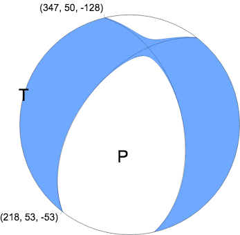
Regional Moment Tensor (Mwr)
Moment 1.179e+16 N-m
Magnitude 4.65 Mwr
Depth 47.0 km
Percent DC 96%
Half Duration -
Catalog US
Data Source US 3
Contributor US 3

Nodal Planes
Plane Strike Dip Rake
NP1 347 50 -128
NP2 218 53 -53

Principal Axes
Axis Value Plunge Azimuth
T 1.168e+16 N-m 1 283
N 0.022e+16 N-m 28 13
P -1.189e+16 N-m 62 191
|
Magnitudes
Given the availability of digital waveforms for determination of the moment tensor, this section documents the added processing leading to mLg, if appropriate to the region, and ML by application of the respective IASPEI formulae. As a research study, the linear distance term of the IASPEI formula
for ML is adjusted to remove a linear distance trend in residuals to give a regionally defined ML. The defined ML uses horizontal component recordings, but the same procedure is applied to the vertical components since there may be some interest in vertical component ground motions. Residual plots versus distance may indicate interesting features of ground motion scaling in some distance ranges. A residual plot of the regionalized magnitude is given as a function of distance and azimuth, since data sets may transcend different wave propagation provinces.
ML Magnitude
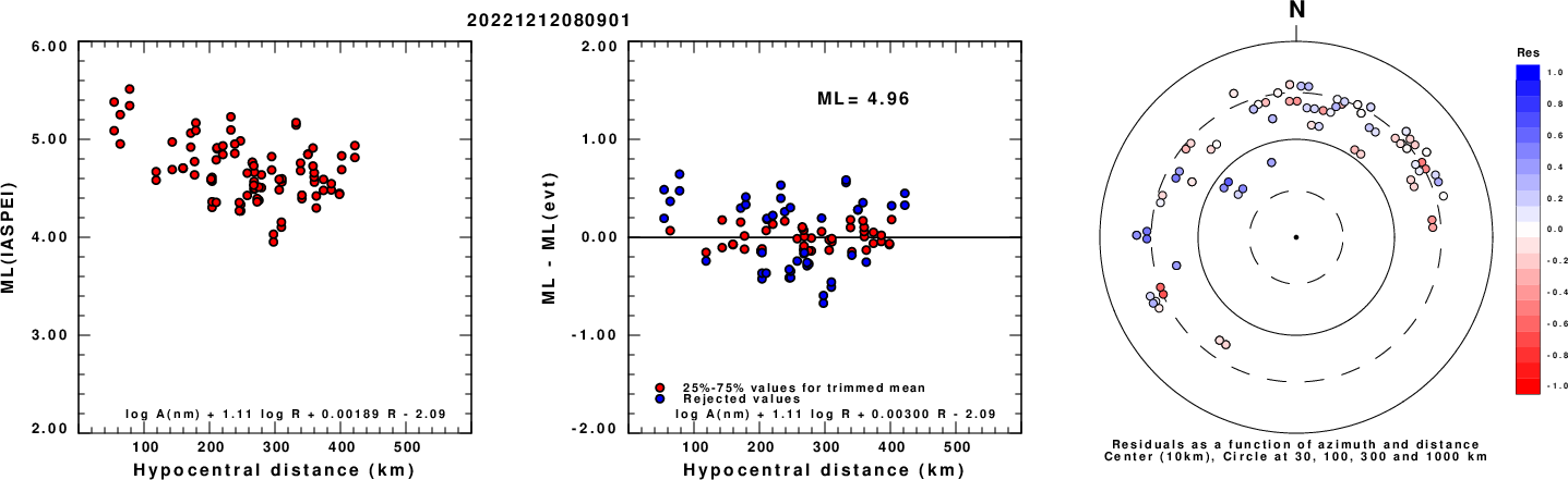
Left: ML computed using the IASPEI formula for Horizontal components. Center: ML residuals computed using a modified IASPEI formula that accounts for path specific attenuation; the values used for the trimmed mean are indicated. The ML relation used for each figure is given at the bottom of each plot.
Right: Residuals from new relation as a function of distance and azimuth.
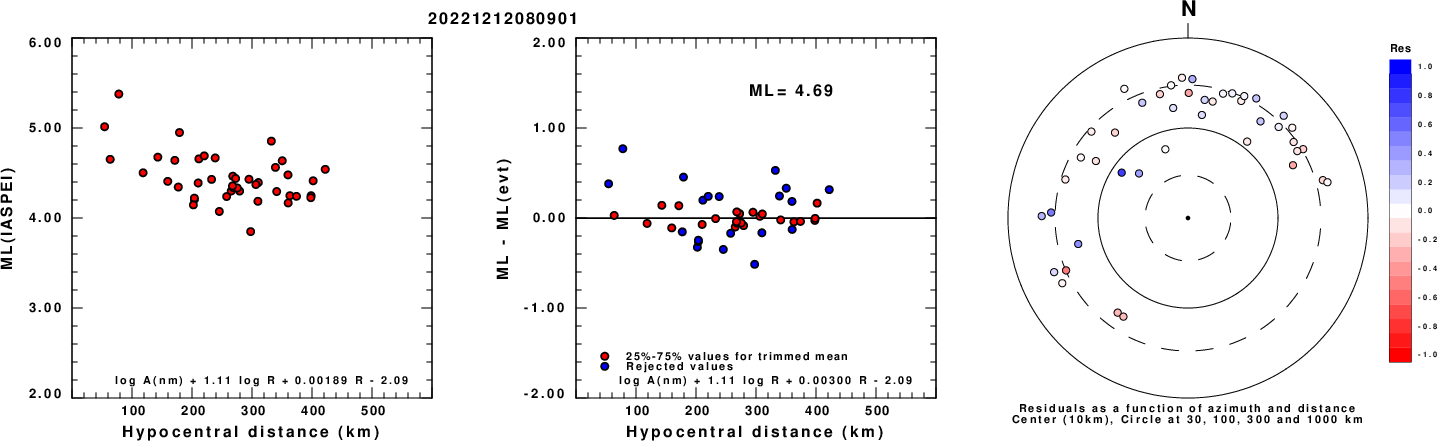
Left: ML computed using the IASPEI formula for Vertical components (research). Center: ML residuals computed using a modified IASPEI formula that accounts for path specific attenuation; the values used for the trimmed mean are indicated. The ML relation used for each figure is given at the bottom of each plot.
Right: Residuals from new relation as a function of distance and azimuth.
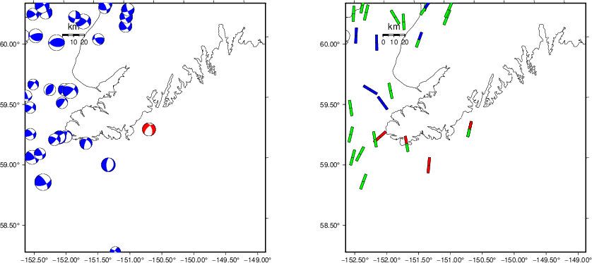
Context
The left panel of the next figure presents the focal mechanism for this earthquake (red) in the context of other nearby events (blue) in the SLU Moment Tensor Catalog. The right panel shows the inferred direction of maximum compressive stress and the type of faulting (green is strike-slip, red is normal, blue is thrust; oblique is shown by a combination of colors). Thus context plot is useful for assessing the appropriateness of the moment tensor of this event.
Waveform Inversion using wvfgrd96
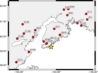
The focal mechanism was determined using broadband seismic waveforms. The location of the event (star) and the
stations used for (red) the waveform inversion are shown in the next figure.
|
|
Location of broadband stations used for waveform inversion
|
The program wvfgrd96 was used with good traces observed at short distance to determine the focal mechanism, depth and seismic moment. This technique requires a high quality signal and well determined velocity model for the Green's functions. To the extent that these are the quality data, this type of mechanism should be preferred over the radiation pattern technique which requires the separate step of defining the pressure and tension quadrants and the correct strike.
The observed and predicted traces are filtered using the following gsac commands:
cut o DIST/3.3 -40 o DIST/3.3 +50
rtr
taper w 0.1
hp c 0.03 n 3
lp c 0.08 n 3
The results of this grid search are as follow:
           DEPTH  STK   DIP  RAKE   MW    FIT
WVFGRD96    1.0   200    60    35   3.86 0.2251
WVFGRD96    2.0    45    45    70   4.02 0.2892
WVFGRD96    3.0    10    45   -90   4.08 0.2849
WVFGRD96    4.0   185    70   -35   4.07 0.2938
WVFGRD96    5.0   190    75   -35   4.08 0.3209
WVFGRD96    6.0    50    90    45   4.07 0.3424
WVFGRD96    7.0    50    90    40   4.09 0.3658
WVFGRD96    8.0    55    85    45   4.16 0.3847
WVFGRD96    9.0   230    90   -45   4.17 0.4006
WVFGRD96   10.0   230    90   -40   4.18 0.4142
WVFGRD96   11.0    55    80    40   4.20 0.4258
WVFGRD96   12.0   230    90   -40   4.21 0.4338
WVFGRD96   13.0   230    90   -40   4.23 0.4409
WVFGRD96   14.0    55    85    35   4.25 0.4478
WVFGRD96   15.0   230    90   -35   4.26 0.4539
WVFGRD96   16.0    55    85    35   4.27 0.4595
WVFGRD96   17.0    50    90    35   4.28 0.4645
WVFGRD96   18.0   230    85   -35   4.30 0.4723
WVFGRD96   19.0   230    85   -35   4.31 0.4795
WVFGRD96   20.0   230    85   -35   4.32 0.4866
WVFGRD96   21.0   230    85   -35   4.33 0.4924
WVFGRD96   22.0   230    80   -35   4.35 0.4976
WVFGRD96   23.0   230    80   -35   4.35 0.5034
WVFGRD96   24.0   230    80   -35   4.36 0.5084
WVFGRD96   25.0   230    80   -35   4.37 0.5118
WVFGRD96   26.0   225    70   -35   4.38 0.5163
WVFGRD96   27.0   230    70   -35   4.40 0.5205
WVFGRD96   28.0   225    65   -35   4.40 0.5246
WVFGRD96   29.0   225    65   -35   4.41 0.5287
WVFGRD96   30.0   230    75   -35   4.41 0.5364
WVFGRD96   31.0   230    75   -35   4.42 0.5483
WVFGRD96   32.0   230    70   -35   4.44 0.5614
WVFGRD96   33.0   225    65   -40   4.44 0.5760
WVFGRD96   34.0   225    65   -40   4.45 0.5899
WVFGRD96   35.0   225    65   -40   4.46 0.6017
WVFGRD96   36.0   230    65   -40   4.48 0.6129
WVFGRD96   37.0   230    65   -40   4.49 0.6226
WVFGRD96   38.0   225    60   -40   4.49 0.6333
WVFGRD96   39.0   225    60   -40   4.50 0.6390
WVFGRD96   40.0   225    60   -45   4.59 0.6510
WVFGRD96   41.0   225    60   -45   4.60 0.6557
WVFGRD96   42.0   225    60   -45   4.61 0.6598
WVFGRD96   43.0   225    60   -45   4.62 0.6611
WVFGRD96   44.0   225    60   -45   4.62 0.6632
WVFGRD96   45.0   220    55   -50   4.63 0.6627
WVFGRD96   46.0   220    55   -50   4.64 0.6615
WVFGRD96   47.0   220    55   -50   4.64 0.6601
WVFGRD96   48.0   220    55   -50   4.65 0.6583
WVFGRD96   49.0   225    55   -45   4.65 0.6562
WVFGRD96   50.0   225    55   -45   4.65 0.6539
WVFGRD96   51.0   225    55   -45   4.66 0.6512
WVFGRD96   52.0   225    55   -45   4.66 0.6483
WVFGRD96   53.0   225    55   -45   4.66 0.6444
WVFGRD96   54.0   225    55   -45   4.66 0.6406
WVFGRD96   55.0   225    55   -45   4.67 0.6366
WVFGRD96   56.0   225    55   -45   4.67 0.6323
WVFGRD96   57.0   220    50   -45   4.67 0.6278
WVFGRD96   58.0   220    50   -45   4.67 0.6237
WVFGRD96   59.0   225    50   -45   4.68 0.6181
The best solution is
WVFGRD96 44.0 225 60 -45 4.62 0.6632
The mechanism corresponding to the best fit is
|
|
Figure 1. Waveform inversion focal mechanism
|
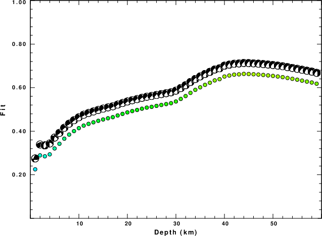
The best fit as a function of depth is given in the following figure:
|
|
Figure 2. Depth sensitivity for waveform mechanism
|
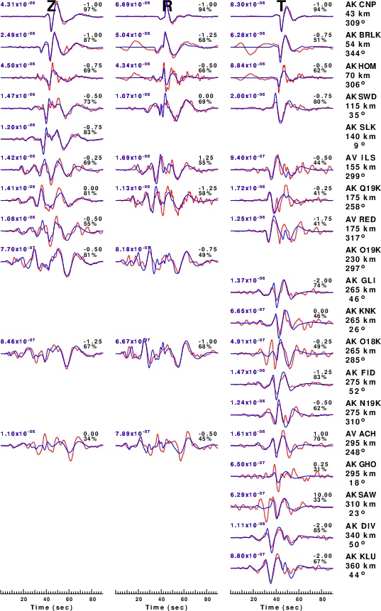
The comparison of the observed and predicted waveforms is given in the next figure. The red traces are the observed and the blue are the predicted.
Each observed-predicted component is plotted to the same scale and peak amplitudes are indicated by the numbers to the left of each trace. A pair of numbers is given in black at the right of each predicted traces. The upper number it the time shift required for maximum correlation between the observed and predicted traces. This time shift is required because the synthetics are not computed at exactly the same distance as the observed, the velocity model used in the predictions may not be perfect and the epicentral parameters may be be off.
A positive time shift indicates that the prediction is too fast and should be delayed to match the observed trace (shift to the right in this figure). A negative value indicates that the prediction is too slow. The lower number gives the percentage of variance reduction to characterize the individual goodness of fit (100% indicates a perfect fit).
The bandpass filter used in the processing and for the display was
cut o DIST/3.3 -40 o DIST/3.3 +50
rtr
taper w 0.1
hp c 0.03 n 3
lp c 0.08 n 3
|
|
Figure 3. Waveform comparison for selected depth. Red: observed; Blue - predicted. The time shift with respect to the model prediction is indicated. The percent of fit is also indicated. The time scale is relative to the first trace sample.
|
|
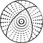
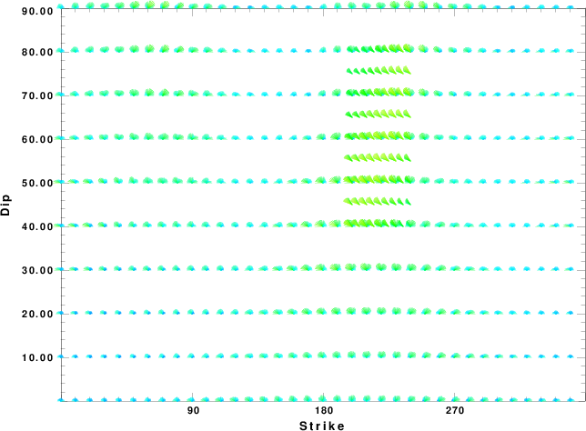
|
Focal mechanism sensitivity at the preferred depth. The red color indicates a very good fit to the waveforms.
Each solution is plotted as a vector at a given value of strike and dip with the angle of the vector representing the rake angle, measured, with respect to the upward vertical (N) in the figure.
|
A check on the assumed source location is possible by looking at the time shifts between the observed and predicted traces. The time shifts for waveform matching arise for several reasons:
- The origin time and epicentral distance are incorrect
- The velocity model used for the inversion is incorrect
- The velocity model used to define the P-arrival time is not the
same as the velocity model used for the waveform inversion
(assuming that the initial trace alignment is based on the
P arrival time)
Assuming only a mislocation, the time shifts are fit to a functional form:
Time_shift = A + B cos Azimuth + C Sin Azimuth
The time shifts for this inversion lead to the next figure:
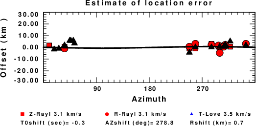
The derived shift in origin time and epicentral coordinates are given at the bottom of the figure.
Velocity Model
The WUS.model used for the waveform synthetic seismograms and for the surface wave eigenfunctions and dispersion is as follows
(The format is in the model96 format of Computer Programs in Seismology).
MODEL.01
Model after     8 iterations
ISOTROPIC
KGS
FLAT EARTH
1-D
CONSTANT VELOCITY
LINE08
LINE09
LINE10
LINE11
      H(KM)   VP(KM/S)   VS(KM/S) RHO(GM/CC)         QP         QS       ETAP       ETAS      FREFP      FREFS
     1.9000     3.4065     2.0089     2.2150  0.302E-02  0.679E-02   0.00       0.00       1.00       1.00
     6.1000     5.5445     3.2953     2.6089  0.349E-02  0.784E-02   0.00       0.00       1.00       1.00
    13.0000     6.2708     3.7396     2.7812  0.212E-02  0.476E-02   0.00       0.00       1.00       1.00
    19.0000     6.4075     3.7680     2.8223  0.111E-02  0.249E-02   0.00       0.00       1.00       1.00
     0.0000     7.9000     4.6200     3.2760  0.164E-10  0.370E-10   0.00       0.00       1.00       1.00
Last Changed Thu Apr 25 03:38:16 AM CDT 2024