Location
Location ANSS
The ANSS event ID is us7000ishe and the event page is at
https://earthquake.usgs.gov/earthquakes/eventpage/us7000ishe/executive.
2022/11/26 03:50:16 49.271 -126.092 33.4 4.9 BC, Canada
Focal Mechanism
 USGS/SLU Moment Tensor Solution
 ENS  2022/11/26 03:50:16:0  49.27 -126.09  33.4 4.9 BC, Canada

 Stations used:
   C8.BCOV CN.BPEB CN.CBB CN.CLRS CN.FHBB CN.GDR CN.MGRB
   CN.NLLB CN.NTKA CN.OZB CN.PABB CN.PACB CN.PGC CN.PHC
   CN.PTRF CN.SYMB CN.TAHB CN.TXDB CN.VDEB CN.VGZ CN.WOSB
   CN.WSLR PQ.ALBHB UW.BHAM UW.CROWN UW.DONK UW.HDW UW.LRIV
   UW.MULN UW.OHOH UW.OTR UW.RNWY UW.SAXON UW.SLDQ UW.SNAG

 Filtering commands used:
   cut o DIST/3.3 -40 o DIST/3.3 +50
   rtr
   taper w 0.1
   hp c 0.03 n 3
   lp c 0.07 n 3

 Best Fitting Double Couple
  Mo = 1.46e+23 dyne-cm
  Mw = 4.71
  Z  = 33 km
  Plane   Strike  Dip  Rake
   NP1      323    81   -160
   NP2      230    70   -10
  Principal Axes:
   Axis    Value   Plunge  Azimuth
    T   1.46e+23      7      95
    N   0.00e+00     68     347
    P  -1.46e+23     21     188

 Moment Tensor: (dyne-cm)
    Component   Value
       Mxx    -1.24e+23
       Mxy    -3.15e+22
       Mxz     4.66e+22
       Myy     1.40e+23
       Myz     2.52e+22
       Mzz    -1.63e+22


                     --------------
                 ----------------------
              ###-------------------------
             ######------------------------
           ##########-----------------#######
          #############-----------############
         ###############-------################
        ##################--####################
        ##################-#####################
       ################------####################
       ##############---------################
       #############------------############## T
       ###########---------------#############
        #########-----------------##############
        #######--------------------#############
         #####----------------------###########
          ###------------------------#########
           #--------------------------#######
             -----------   ------------####
              ---------- P -------------##
                 -------   ------------
                     --------------


 Global CMT Convention Moment Tensor:
      R          T          P
 -1.63e+22   4.66e+22  -2.52e+22
  4.66e+22  -1.24e+23   3.15e+22
 -2.52e+22   3.15e+22   1.40e+23


Details of the solution is found at

http://www.eas.slu.edu/eqc/eqc_mt/MECH.NA/20221126035016/index.html
|
Preferred Solution
The preferred solution from an analysis of the surface-wave spectral amplitude radiation pattern, waveform inversion or first motion observations is
      STK = 230
      DIP = 70
     RAKE = -10
       MW = 4.71
       HS = 33.0
The NDK file is 20221126035016.ndk
The waveform inversion is preferred.
Magnitudes
Given the availability of digital waveforms for determination of the moment tensor, this section documents the added processing leading to mLg, if appropriate to the region, and ML by application of the respective IASPEI formulae. As a research study, the linear distance term of the IASPEI formula
for ML is adjusted to remove a linear distance trend in residuals to give a regionally defined ML. The defined ML uses horizontal component recordings, but the same procedure is applied to the vertical components since there may be some interest in vertical component ground motions. Residual plots versus distance may indicate interesting features of ground motion scaling in some distance ranges. A residual plot of the regionalized magnitude is given as a function of distance and azimuth, since data sets may transcend different wave propagation provinces.
ML Magnitude
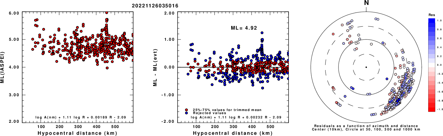
Left: ML computed using the IASPEI formula for Horizontal components. Center: ML residuals computed using a modified IASPEI formula that accounts for path specific attenuation; the values used for the trimmed mean are indicated. The ML relation used for each figure is given at the bottom of each plot.
Right: Residuals from new relation as a function of distance and azimuth.
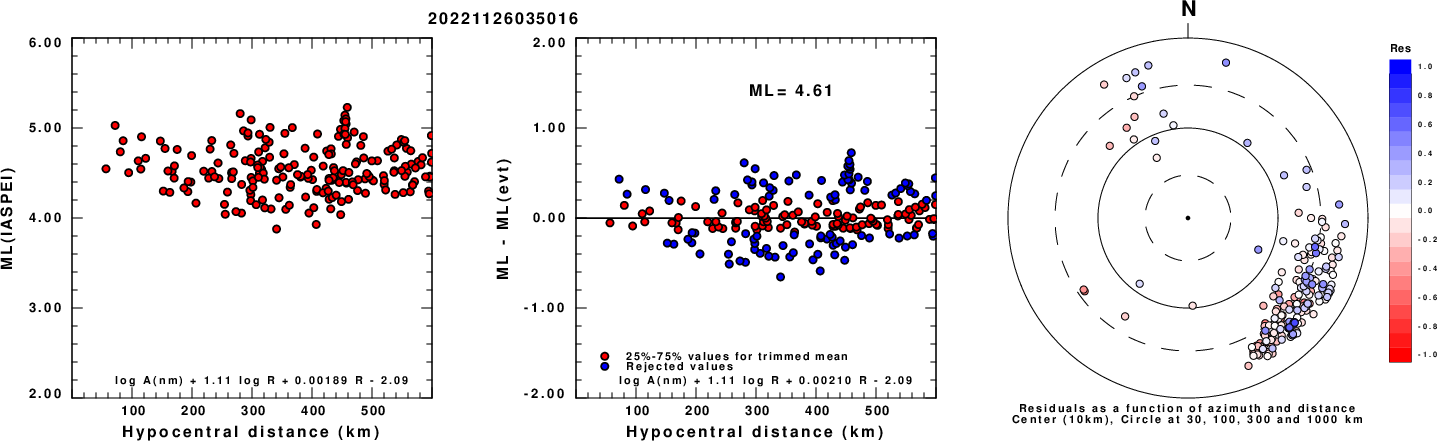
Left: ML computed using the IASPEI formula for Vertical components (research). Center: ML residuals computed using a modified IASPEI formula that accounts for path specific attenuation; the values used for the trimmed mean are indicated. The ML relation used for each figure is given at the bottom of each plot.
Right: Residuals from new relation as a function of distance and azimuth.
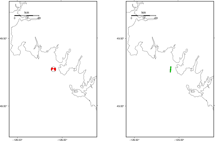
Context
The left panel of the next figure presents the focal mechanism for this earthquake (red) in the context of other nearby events (blue) in the SLU Moment Tensor Catalog. The right panel shows the inferred direction of maximum compressive stress and the type of faulting (green is strike-slip, red is normal, blue is thrust; oblique is shown by a combination of colors). Thus context plot is useful for assessing the appropriateness of the moment tensor of this event.
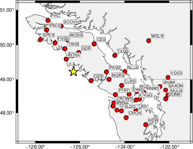
Waveform Inversion using wvfgrd96
The focal mechanism was determined using broadband seismic waveforms. The location of the event (star) and the
stations used for (red) the waveform inversion are shown in the next figure.
|
|
Location of broadband stations used for waveform inversion
|
The program wvfgrd96 was used with good traces observed at short distance to determine the focal mechanism, depth and seismic moment. This technique requires a high quality signal and well determined velocity model for the Green's functions. To the extent that these are the quality data, this type of mechanism should be preferred over the radiation pattern technique which requires the separate step of defining the pressure and tension quadrants and the correct strike.
The observed and predicted traces are filtered using the following gsac commands:
cut o DIST/3.3 -40 o DIST/3.3 +50
rtr
taper w 0.1
hp c 0.03 n 3
lp c 0.07 n 3
The results of this grid search are as follow:
           DEPTH  STK   DIP  RAKE   MW    FIT
WVFGRD96    1.0   320    75   -15   4.05 0.2179
WVFGRD96    2.0   320    75   -20   4.17 0.2872
WVFGRD96    3.0   320    75   -15   4.22 0.3173
WVFGRD96    4.0   320    80   -15   4.25 0.3345
WVFGRD96    5.0   230    80   -20   4.29 0.3446
WVFGRD96    6.0   230    80   -20   4.32 0.3669
WVFGRD96    7.0   230    80   -20   4.35 0.3886
WVFGRD96    8.0   230    80   -20   4.39 0.4121
WVFGRD96    9.0   230    80   -20   4.41 0.4274
WVFGRD96   10.0   230    85   -25   4.42 0.4444
WVFGRD96   11.0   235    90   -25   4.44 0.4624
WVFGRD96   12.0    55    90    20   4.46 0.4804
WVFGRD96   13.0   235    90   -20   4.48 0.4976
WVFGRD96   14.0   230    70   -15   4.50 0.5138
WVFGRD96   15.0   230    70   -15   4.52 0.5340
WVFGRD96   16.0   230    70   -15   4.53 0.5540
WVFGRD96   17.0   230    70   -15   4.54 0.5743
WVFGRD96   18.0   230    70   -10   4.56 0.5934
WVFGRD96   19.0   230    70   -10   4.57 0.6116
WVFGRD96   20.0   230    70   -10   4.59 0.6289
WVFGRD96   21.0   230    70   -10   4.60 0.6445
WVFGRD96   22.0   230    70   -10   4.61 0.6601
WVFGRD96   23.0   230    70   -10   4.62 0.6749
WVFGRD96   24.0   230    70   -10   4.63 0.6887
WVFGRD96   25.0   230    70   -10   4.64 0.7018
WVFGRD96   26.0   230    70   -10   4.65 0.7136
WVFGRD96   27.0   230    70   -10   4.66 0.7233
WVFGRD96   28.0   230    70   -10   4.67 0.7318
WVFGRD96   29.0   230    70   -10   4.68 0.7381
WVFGRD96   30.0   230    70   -10   4.69 0.7421
WVFGRD96   31.0   230    70   -10   4.70 0.7455
WVFGRD96   32.0   230    70   -10   4.71 0.7465
WVFGRD96   33.0   230    70   -10   4.71 0.7467
WVFGRD96   34.0   230    70   -10   4.72 0.7451
WVFGRD96   35.0   230    70   -10   4.73 0.7428
WVFGRD96   36.0   230    70   -10   4.74 0.7401
WVFGRD96   37.0   230    70   -10   4.75 0.7379
WVFGRD96   38.0   230    70   -10   4.77 0.7368
WVFGRD96   39.0   230    70   -10   4.78 0.7371
WVFGRD96   40.0   230    65   -15   4.82 0.7313
WVFGRD96   41.0   230    65   -15   4.83 0.7338
WVFGRD96   42.0   230    65   -15   4.84 0.7344
WVFGRD96   43.0   230    70   -15   4.85 0.7331
WVFGRD96   44.0   230    70   -15   4.85 0.7314
WVFGRD96   45.0   230    70   -15   4.86 0.7288
WVFGRD96   46.0   230    70   -15   4.87 0.7252
WVFGRD96   47.0   230    70   -15   4.87 0.7210
WVFGRD96   48.0   230    70   -10   4.88 0.7169
WVFGRD96   49.0   230    70   -10   4.89 0.7129
WVFGRD96   50.0   230    70   -10   4.89 0.7077
WVFGRD96   51.0   225    65   -10   4.90 0.7037
WVFGRD96   52.0   225    65   -10   4.90 0.6992
WVFGRD96   53.0   225    65   -10   4.91 0.6952
WVFGRD96   54.0   225    65   -10   4.91 0.6902
WVFGRD96   55.0   225    65   -10   4.92 0.6852
WVFGRD96   56.0   225    65   -10   4.92 0.6805
WVFGRD96   57.0   225    65   -10   4.92 0.6753
WVFGRD96   58.0   225    65   -10   4.93 0.6701
WVFGRD96   59.0   225    65   -10   4.93 0.6646
The best solution is
WVFGRD96 33.0 230 70 -10 4.71 0.7467
The mechanism corresponding to the best fit is
|
|
Figure 1. Waveform inversion focal mechanism
|
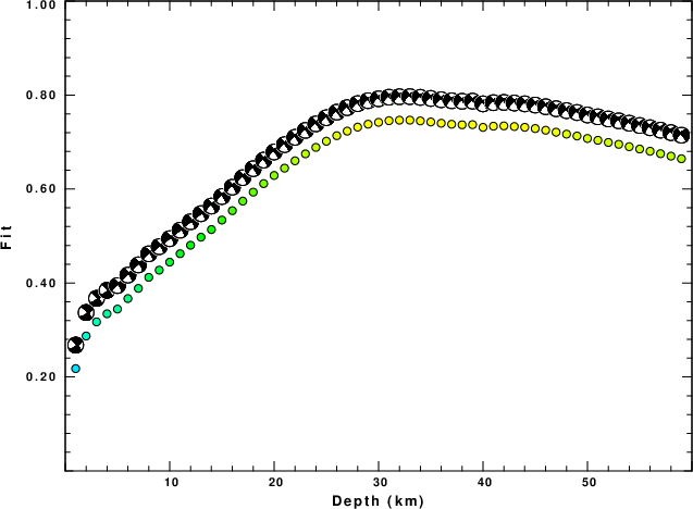
The best fit as a function of depth is given in the following figure:
|
|
Figure 2. Depth sensitivity for waveform mechanism
|
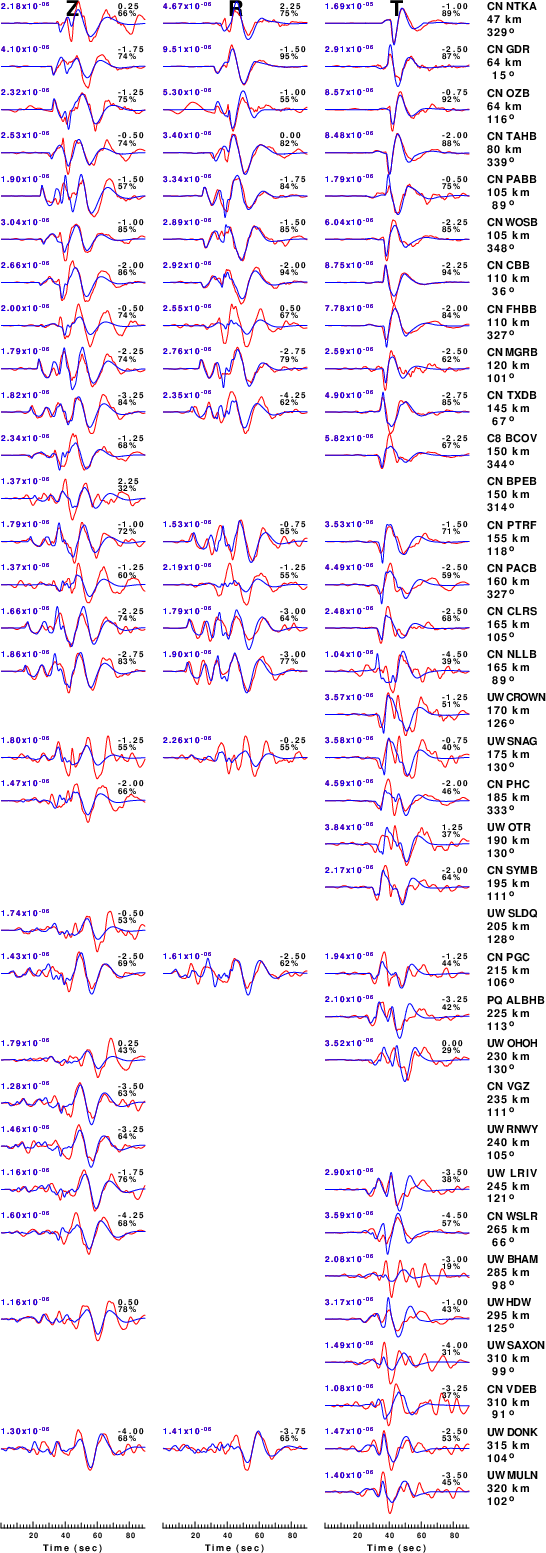
The comparison of the observed and predicted waveforms is given in the next figure. The red traces are the observed and the blue are the predicted.
Each observed-predicted component is plotted to the same scale and peak amplitudes are indicated by the numbers to the left of each trace. A pair of numbers is given in black at the right of each predicted traces. The upper number it the time shift required for maximum correlation between the observed and predicted traces. This time shift is required because the synthetics are not computed at exactly the same distance as the observed, the velocity model used in the predictions may not be perfect and the epicentral parameters may be be off.
A positive time shift indicates that the prediction is too fast and should be delayed to match the observed trace (shift to the right in this figure). A negative value indicates that the prediction is too slow. The lower number gives the percentage of variance reduction to characterize the individual goodness of fit (100% indicates a perfect fit).
The bandpass filter used in the processing and for the display was
cut o DIST/3.3 -40 o DIST/3.3 +50
rtr
taper w 0.1
hp c 0.03 n 3
lp c 0.07 n 3
|
|
Figure 3. Waveform comparison for selected depth. Red: observed; Blue - predicted. The time shift with respect to the model prediction is indicated. The percent of fit is also indicated. The time scale is relative to the first trace sample.
|
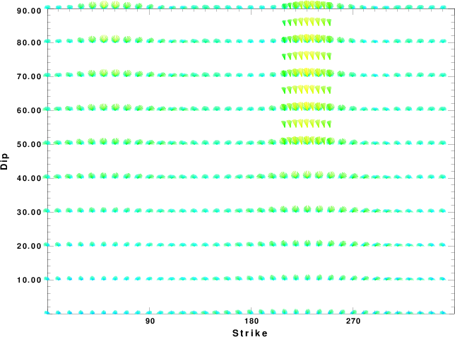
|
|
Focal mechanism sensitivity at the preferred depth. The red color indicates a very good fit to the waveforms.
Each solution is plotted as a vector at a given value of strike and dip with the angle of the vector representing the rake angle, measured, with respect to the upward vertical (N) in the figure.
|
A check on the assumed source location is possible by looking at the time shifts between the observed and predicted traces. The time shifts for waveform matching arise for several reasons:
- The origin time and epicentral distance are incorrect
- The velocity model used for the inversion is incorrect
- The velocity model used to define the P-arrival time is not the
same as the velocity model used for the waveform inversion
(assuming that the initial trace alignment is based on the
P arrival time)
Assuming only a mislocation, the time shifts are fit to a functional form:
Time_shift = A + B cos Azimuth + C Sin Azimuth
The time shifts for this inversion lead to the next figure:
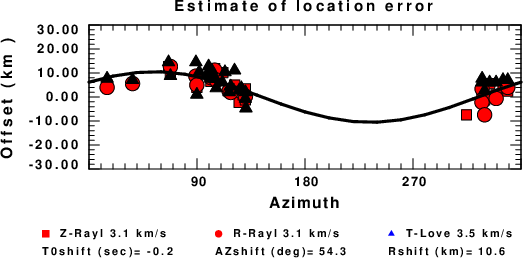
The derived shift in origin time and epicentral coordinates are given at the bottom of the figure.
Velocity Model
The WUS.model used for the waveform synthetic seismograms and for the surface wave eigenfunctions and dispersion is as follows
(The format is in the model96 format of Computer Programs in Seismology).
MODEL.01
Model after     8 iterations
ISOTROPIC
KGS
FLAT EARTH
1-D
CONSTANT VELOCITY
LINE08
LINE09
LINE10
LINE11
      H(KM)   VP(KM/S)   VS(KM/S) RHO(GM/CC)         QP         QS       ETAP       ETAS      FREFP      FREFS
     1.9000     3.4065     2.0089     2.2150  0.302E-02  0.679E-02   0.00       0.00       1.00       1.00
     6.1000     5.5445     3.2953     2.6089  0.349E-02  0.784E-02   0.00       0.00       1.00       1.00
    13.0000     6.2708     3.7396     2.7812  0.212E-02  0.476E-02   0.00       0.00       1.00       1.00
    19.0000     6.4075     3.7680     2.8223  0.111E-02  0.249E-02   0.00       0.00       1.00       1.00
     0.0000     7.9000     4.6200     3.2760  0.164E-10  0.370E-10   0.00       0.00       1.00       1.00
Last Changed Thu Apr 25 03:10:52 AM CDT 2024