Location
SLU Location
To check the ANSS location or to compare the observed P-wave first motions to the moment tensor solution, P- and S-wave first arrival times were manually read together with the P-wave first motions. The subsequent output of the program elocate is given in the file elocate.txt. The first motion plot is shown below.
Location ANSS
The ANSS event ID is ak022ctqflju and the event page is at
https://earthquake.usgs.gov/earthquakes/eventpage/ak022ctqflju/executive.
2022/10/06 19:30:50 61.850 -147.578 28.7 4.1 Alaska
Focal Mechanism
 USGS/SLU Moment Tensor Solution
 ENS  2022/10/06 19:30:50:0  61.85 -147.58  28.7 4.1 Alaska

 Stations used:
   AK.BMR AK.CCB AK.CUT AK.DHY AK.EYAK AK.FID AK.GHO AK.GLI
   AK.HDA AK.HIN AK.K24K AK.KLU AK.KNK AK.L22K AK.MCAR AK.MCK
   AK.POKR AK.PWL AK.RC01 AK.SAW AK.SCM AK.SKN AK.SLK AT.PMR
   IM.IL31 IU.COLA

 Filtering commands used:
   cut o DIST/3.3 -40 o DIST/3.3 +50
   rtr
   taper w 0.1
   hp c 0.03 n 3
   lp c 0.08 n 3

 Best Fitting Double Couple
  Mo = 1.66e+22 dyne-cm
  Mw = 4.08
  Z  = 71 km
  Plane   Strike  Dip  Rake
   NP1      360    85   175
   NP2       90    85     5
  Principal Axes:
   Axis    Value   Plunge  Azimuth
    T   1.66e+22      7     315
    N   0.00e+00     83     135
    P  -1.66e+22      0      45

 Moment Tensor: (dyne-cm)
    Component   Value
       Mxx    -2.51e+20
       Mxy    -1.65e+22
       Mxz     1.42e+21
       Myy    -1.44e+15
       Myz    -1.44e+21
       Mzz     2.51e+20


                     #######-------
                 ###########-----------
                #############----------- P
              T #############-----------
           ##   #############----------------
          ###################-----------------
         ####################------------------
        #####################-------------------
        #####################-------------------
       ######################--------------------
       ######################--------------------
       ---------#############-----------#########
       ----------------------####################
        ---------------------###################
        ---------------------###################
         --------------------##################
          -------------------#################
           ------------------################
             ----------------##############
              ---------------#############
                 ------------##########
                     -------#######


 Global CMT Convention Moment Tensor:
      R          T          P
  2.51e+20   1.42e+21   1.44e+21
  1.42e+21  -2.51e+20   1.65e+22
  1.44e+21   1.65e+22  -1.44e+15


Details of the solution is found at

http://www.eas.slu.edu/eqc/eqc_mt/MECH.NA/20221006193050/index.html
|
Preferred Solution
The preferred solution from an analysis of the surface-wave spectral amplitude radiation pattern, waveform inversion or first motion observations is
      STK = 90
      DIP = 85
     RAKE = 5
       MW = 4.08
       HS = 71.0
The NDK file is 20221006193050.ndk
The waveform inversion is preferred.
Moment Tensor Comparison
The following compares this source inversion to those provided by others. The purpose is to look for major differences and also to note slight differences that might be inherent to the processing procedure. For completeness the USGS/SLU solution is repeated from above.
| SLU |
SLUFM |
 USGS/SLU Moment Tensor Solution
 ENS  2022/10/06 19:30:50:0  61.85 -147.58  28.7 4.1 Alaska

 Stations used:
   AK.BMR AK.CCB AK.CUT AK.DHY AK.EYAK AK.FID AK.GHO AK.GLI
   AK.HDA AK.HIN AK.K24K AK.KLU AK.KNK AK.L22K AK.MCAR AK.MCK
   AK.POKR AK.PWL AK.RC01 AK.SAW AK.SCM AK.SKN AK.SLK AT.PMR
   IM.IL31 IU.COLA

 Filtering commands used:
   cut o DIST/3.3 -40 o DIST/3.3 +50
   rtr
   taper w 0.1
   hp c 0.03 n 3
   lp c 0.08 n 3

 Best Fitting Double Couple
  Mo = 1.66e+22 dyne-cm
  Mw = 4.08
  Z  = 71 km
  Plane   Strike  Dip  Rake
   NP1      360    85   175
   NP2       90    85     5
  Principal Axes:
   Axis    Value   Plunge  Azimuth
    T   1.66e+22      7     315
    N   0.00e+00     83     135
    P  -1.66e+22      0      45

 Moment Tensor: (dyne-cm)
    Component   Value
       Mxx    -2.51e+20
       Mxy    -1.65e+22
       Mxz     1.42e+21
       Myy    -1.44e+15
       Myz    -1.44e+21
       Mzz     2.51e+20


                     #######-------
                 ###########-----------
                #############----------- P
              T #############-----------
           ##   #############----------------
          ###################-----------------
         ####################------------------
        #####################-------------------
        #####################-------------------
       ######################--------------------
       ######################--------------------
       ---------#############-----------#########
       ----------------------####################
        ---------------------###################
        ---------------------###################
         --------------------##################
          -------------------#################
           ------------------################
             ----------------##############
              ---------------#############
                 ------------##########
                     -------#######


 Global CMT Convention Moment Tensor:
      R          T          P
  2.51e+20   1.42e+21   1.44e+21
  1.42e+21  -2.51e+20   1.65e+22
  1.44e+21   1.65e+22  -1.44e+15


Details of the solution is found at

http://www.eas.slu.edu/eqc/eqc_mt/MECH.NA/20221006193050/index.html
|
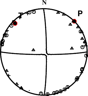
First motions and takeoff angles from an elocate run.
|
Magnitudes
Given the availability of digital waveforms for determination of the moment tensor, this section documents the added processing leading to mLg, if appropriate to the region, and ML by application of the respective IASPEI formulae. As a research study, the linear distance term of the IASPEI formula
for ML is adjusted to remove a linear distance trend in residuals to give a regionally defined ML. The defined ML uses horizontal component recordings, but the same procedure is applied to the vertical components since there may be some interest in vertical component ground motions. Residual plots versus distance may indicate interesting features of ground motion scaling in some distance ranges. A residual plot of the regionalized magnitude is given as a function of distance and azimuth, since data sets may transcend different wave propagation provinces.
ML Magnitude
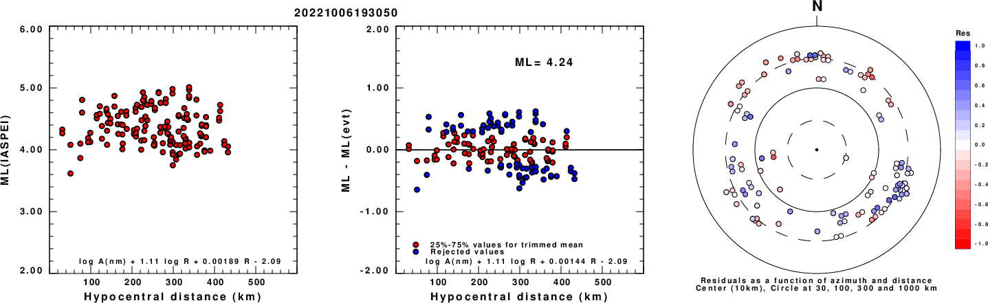
Left: ML computed using the IASPEI formula for Horizontal components. Center: ML residuals computed using a modified IASPEI formula that accounts for path specific attenuation; the values used for the trimmed mean are indicated. The ML relation used for each figure is given at the bottom of each plot.
Right: Residuals from new relation as a function of distance and azimuth.
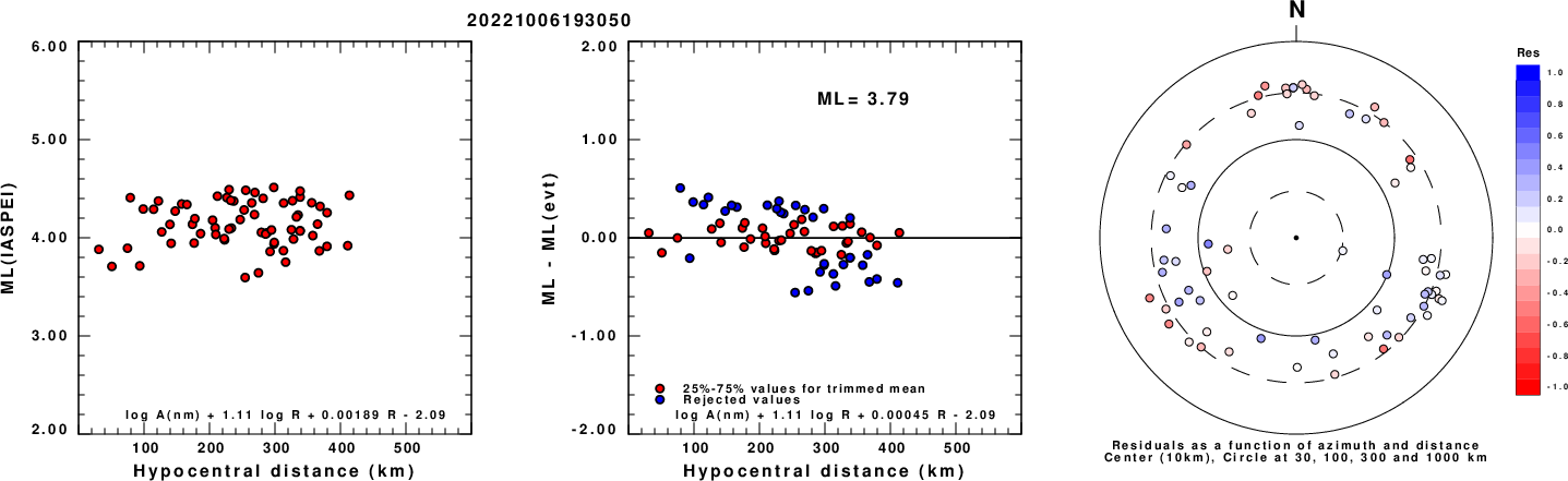
Left: ML computed using the IASPEI formula for Vertical components (research). Center: ML residuals computed using a modified IASPEI formula that accounts for path specific attenuation; the values used for the trimmed mean are indicated. The ML relation used for each figure is given at the bottom of each plot.
Right: Residuals from new relation as a function of distance and azimuth.
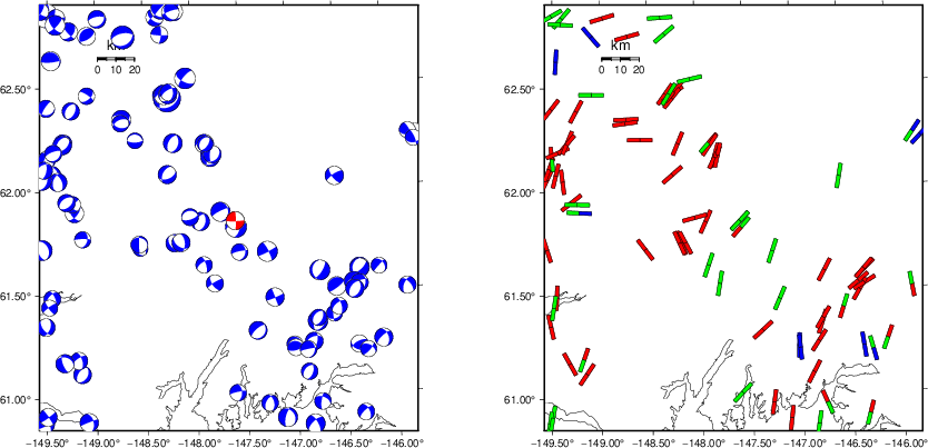
Context
The left panel of the next figure presents the focal mechanism for this earthquake (red) in the context of other nearby events (blue) in the SLU Moment Tensor Catalog. The right panel shows the inferred direction of maximum compressive stress and the type of faulting (green is strike-slip, red is normal, blue is thrust; oblique is shown by a combination of colors). Thus context plot is useful for assessing the appropriateness of the moment tensor of this event.
Waveform Inversion using wvfgrd96
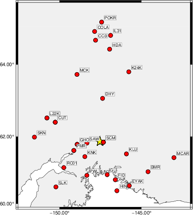
The focal mechanism was determined using broadband seismic waveforms. The location of the event (star) and the
stations used for (red) the waveform inversion are shown in the next figure.
|
|
Location of broadband stations used for waveform inversion
|
The program wvfgrd96 was used with good traces observed at short distance to determine the focal mechanism, depth and seismic moment. This technique requires a high quality signal and well determined velocity model for the Green's functions. To the extent that these are the quality data, this type of mechanism should be preferred over the radiation pattern technique which requires the separate step of defining the pressure and tension quadrants and the correct strike.
The observed and predicted traces are filtered using the following gsac commands:
cut o DIST/3.3 -40 o DIST/3.3 +50
rtr
taper w 0.1
hp c 0.03 n 3
lp c 0.08 n 3
The results of this grid search are as follow:
           DEPTH  STK   DIP  RAKE   MW    FIT
WVFGRD96    1.0    -5    90    15   3.07 0.2284
WVFGRD96    2.0   170    70   -25   3.23 0.3181
WVFGRD96    3.0   175    80   -20   3.27 0.3544
WVFGRD96    4.0   175    85   -20   3.31 0.3795
WVFGRD96    5.0   175    80   -15   3.35 0.3979
WVFGRD96    6.0    -5    90    15   3.37 0.4118
WVFGRD96    7.0    -5    90    15   3.41 0.4241
WVFGRD96    8.0   175    90   -15   3.44 0.4339
WVFGRD96    9.0   175    90   -10   3.46 0.4365
WVFGRD96   10.0   275    70    15   3.51 0.4474
WVFGRD96   11.0   275    70    15   3.54 0.4635
WVFGRD96   12.0   270    75     5   3.54 0.4788
WVFGRD96   13.0   270    75     0   3.56 0.4934
WVFGRD96   14.0   270    75   -10   3.58 0.5080
WVFGRD96   15.0   270    75   -10   3.60 0.5227
WVFGRD96   16.0   270    75   -10   3.62 0.5373
WVFGRD96   17.0   270    75   -10   3.64 0.5521
WVFGRD96   18.0   270    75   -10   3.65 0.5662
WVFGRD96   19.0   270    75   -10   3.67 0.5807
WVFGRD96   20.0   270    75   -10   3.68 0.5955
WVFGRD96   21.0   270    75   -10   3.70 0.6095
WVFGRD96   22.0   270    75   -10   3.71 0.6219
WVFGRD96   23.0   270    75   -10   3.72 0.6348
WVFGRD96   24.0   270    75   -10   3.73 0.6459
WVFGRD96   25.0   270    75   -10   3.74 0.6554
WVFGRD96   26.0   270    75   -10   3.75 0.6634
WVFGRD96   27.0   270    75   -10   3.76 0.6695
WVFGRD96   28.0   270    75   -10   3.77 0.6764
WVFGRD96   29.0   270    75   -10   3.78 0.6808
WVFGRD96   30.0   270    75   -10   3.78 0.6843
WVFGRD96   31.0   270    75   -10   3.79 0.6853
WVFGRD96   32.0   270    75   -10   3.80 0.6850
WVFGRD96   33.0   270    75   -10   3.81 0.6842
WVFGRD96   34.0   270    75   -10   3.82 0.6821
WVFGRD96   35.0   270    75   -10   3.82 0.6798
WVFGRD96   36.0   270    80   -10   3.83 0.6775
WVFGRD96   37.0   270    80   -10   3.85 0.6764
WVFGRD96   38.0   270    75    -5   3.86 0.6768
WVFGRD96   39.0   270    80    -5   3.87 0.6789
WVFGRD96   40.0   270    75   -15   3.91 0.6868
WVFGRD96   41.0   270    75   -15   3.93 0.6885
WVFGRD96   42.0   270    75   -15   3.94 0.6891
WVFGRD96   43.0   270    75   -15   3.95 0.6900
WVFGRD96   44.0   270    75   -15   3.96 0.6901
WVFGRD96   45.0   270    75   -15   3.97 0.6900
WVFGRD96   46.0   270    75   -15   3.98 0.6892
WVFGRD96   47.0   270    75   -15   3.98 0.6877
WVFGRD96   48.0   270    75   -15   3.99 0.6880
WVFGRD96   49.0   270    75   -10   3.99 0.6880
WVFGRD96   50.0   270    75   -10   4.00 0.6887
WVFGRD96   51.0   270    75   -10   4.00 0.6891
WVFGRD96   52.0   270    75   -10   4.01 0.6910
WVFGRD96   53.0   270    75   -10   4.01 0.6912
WVFGRD96   54.0   270    75   -10   4.02 0.6914
WVFGRD96   55.0   270    75   -10   4.03 0.6924
WVFGRD96   56.0   270    75   -10   4.03 0.6917
WVFGRD96   57.0   270    80   -10   4.03 0.6925
WVFGRD96   58.0   270    80   -10   4.04 0.6928
WVFGRD96   59.0   270    80   -10   4.04 0.6925
WVFGRD96   60.0   270    80   -10   4.05 0.6931
WVFGRD96   61.0   270    80   -10   4.05 0.6915
WVFGRD96   62.0   270    80    -5   4.05 0.6920
WVFGRD96   63.0   270    80    -5   4.05 0.6933
WVFGRD96   64.0   270    90    -5   4.05 0.6917
WVFGRD96   65.0    90    85     5   4.06 0.6934
WVFGRD96   66.0    90    85     5   4.06 0.6936
WVFGRD96   67.0    90    85     5   4.06 0.6934
WVFGRD96   68.0    90    85     5   4.07 0.6933
WVFGRD96   69.0    90    85     5   4.07 0.6939
WVFGRD96   70.0    90    85     5   4.07 0.6940
WVFGRD96   71.0    90    85     5   4.08 0.6945
WVFGRD96   72.0    90    85     5   4.08 0.6932
WVFGRD96   73.0    90    85     5   4.08 0.6941
WVFGRD96   74.0    90    85     5   4.09 0.6934
WVFGRD96   75.0    90    85     5   4.09 0.6940
WVFGRD96   76.0    90    85     5   4.09 0.6929
WVFGRD96   77.0    90    85     5   4.09 0.6933
WVFGRD96   78.0    90    85     5   4.10 0.6931
WVFGRD96   79.0    90    85     5   4.10 0.6938
The best solution is
WVFGRD96 71.0 90 85 5 4.08 0.6945
The mechanism corresponding to the best fit is
|
|
Figure 1. Waveform inversion focal mechanism
|
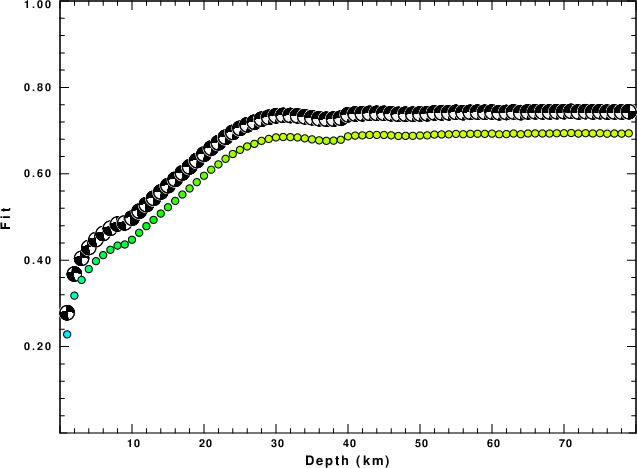
The best fit as a function of depth is given in the following figure:
|
|
Figure 2. Depth sensitivity for waveform mechanism
|
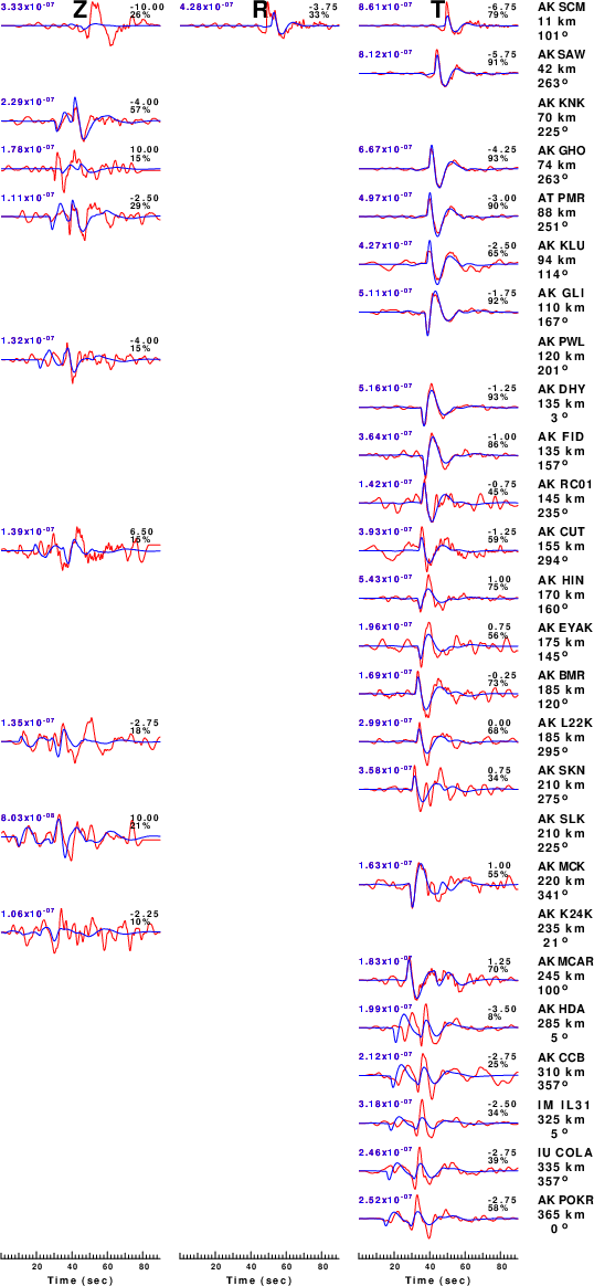
The comparison of the observed and predicted waveforms is given in the next figure. The red traces are the observed and the blue are the predicted.
Each observed-predicted component is plotted to the same scale and peak amplitudes are indicated by the numbers to the left of each trace. A pair of numbers is given in black at the right of each predicted traces. The upper number it the time shift required for maximum correlation between the observed and predicted traces. This time shift is required because the synthetics are not computed at exactly the same distance as the observed, the velocity model used in the predictions may not be perfect and the epicentral parameters may be be off.
A positive time shift indicates that the prediction is too fast and should be delayed to match the observed trace (shift to the right in this figure). A negative value indicates that the prediction is too slow. The lower number gives the percentage of variance reduction to characterize the individual goodness of fit (100% indicates a perfect fit).
The bandpass filter used in the processing and for the display was
cut o DIST/3.3 -40 o DIST/3.3 +50
rtr
taper w 0.1
hp c 0.03 n 3
lp c 0.08 n 3
|
|
Figure 3. Waveform comparison for selected depth. Red: observed; Blue - predicted. The time shift with respect to the model prediction is indicated. The percent of fit is also indicated. The time scale is relative to the first trace sample.
|
|
|
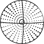
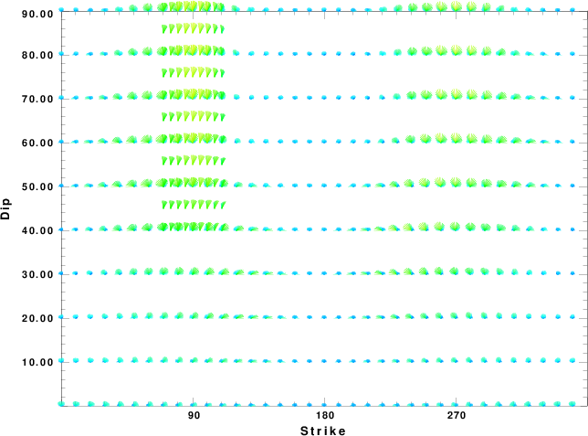
Focal mechanism sensitivity at the preferred depth. The red color indicates a very good fit to the waveforms.
Each solution is plotted as a vector at a given value of strike and dip with the angle of the vector representing the rake angle, measured, with respect to the upward vertical (N) in the figure.
|
A check on the assumed source location is possible by looking at the time shifts between the observed and predicted traces. The time shifts for waveform matching arise for several reasons:
- The origin time and epicentral distance are incorrect
- The velocity model used for the inversion is incorrect
- The velocity model used to define the P-arrival time is not the
same as the velocity model used for the waveform inversion
(assuming that the initial trace alignment is based on the
P arrival time)
Assuming only a mislocation, the time shifts are fit to a functional form:
Time_shift = A + B cos Azimuth + C Sin Azimuth
The time shifts for this inversion lead to the next figure:
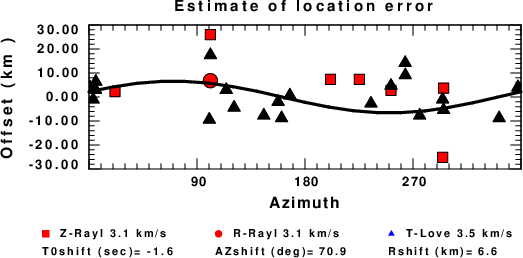
The derived shift in origin time and epicentral coordinates are given at the bottom of the figure.
Velocity Model
The WUS.model used for the waveform synthetic seismograms and for the surface wave eigenfunctions and dispersion is as follows
(The format is in the model96 format of Computer Programs in Seismology).
MODEL.01
Model after     8 iterations
ISOTROPIC
KGS
FLAT EARTH
1-D
CONSTANT VELOCITY
LINE08
LINE09
LINE10
LINE11
      H(KM)   VP(KM/S)   VS(KM/S) RHO(GM/CC)         QP         QS       ETAP       ETAS      FREFP      FREFS
     1.9000     3.4065     2.0089     2.2150  0.302E-02  0.679E-02   0.00       0.00       1.00       1.00
     6.1000     5.5445     3.2953     2.6089  0.349E-02  0.784E-02   0.00       0.00       1.00       1.00
    13.0000     6.2708     3.7396     2.7812  0.212E-02  0.476E-02   0.00       0.00       1.00       1.00
    19.0000     6.4075     3.7680     2.8223  0.111E-02  0.249E-02   0.00       0.00       1.00       1.00
     0.0000     7.9000     4.6200     3.2760  0.164E-10  0.370E-10   0.00       0.00       1.00       1.00
Last Changed Thu Apr 25 01:48:43 AM CDT 2024