Location
Location ANSS
The ANSS event ID is ak022crxd45r and the event page is at
https://earthquake.usgs.gov/earthquakes/eventpage/ak022crxd45r/executive.
2022/10/05 10:01:40 61.748 -149.768 42.5 3.7 Alaska
Focal Mechanism
 USGS/SLU Moment Tensor Solution
 ENS  2022/10/05 10:01:40:0  61.75 -149.77  42.5 3.7 Alaska

 Stations used:
   AK.CUT AK.DHY AK.FIRE AK.GHO AK.GLI AK.KNK AK.RC01 AK.SAW
   AK.SCM AK.SSN AT.PMR

 Filtering commands used:
   cut o DIST/3.3 -40 o DIST/3.3 +50
   rtr
   taper w 0.1
   hp c 0.03 n 3
   lp c 0.08 n 3

 Best Fitting Double Couple
  Mo = 7.00e+21 dyne-cm
  Mw = 3.83
  Z  = 49 km
  Plane   Strike  Dip  Rake
   NP1      275    55   -50
   NP2       39    51   -133
  Principal Axes:
   Axis    Value   Plunge  Azimuth
    T   7.00e+21      2     338
    N   0.00e+00     32      69
    P  -7.00e+21     58     244

 Moment Tensor: (dyne-cm)
    Component   Value
       Mxx     5.64e+21
       Mxy    -3.19e+21
       Mxz     1.60e+21
       Myy    -6.02e+20
       Myz     2.73e+21
       Mzz    -5.04e+21


                     T ############
                 ###   ################
              ###########################-
             #############################-
           ###############################---
          ################################----
         ##########-------------##########-----
        ######------------------------####------
        ##-------------------------------#------
       #---------------------------------####----
       ---------------------------------#######--
       ------------   -----------------#########-
       ------------ P ----------------###########
        -----------   ---------------###########
        ---------------------------#############
         -------------------------#############
          ----------------------##############
           ------------------################
             -------------#################
              -------#####################
                 ######################
                     ##############


 Global CMT Convention Moment Tensor:
      R          T          P
 -5.04e+21   1.60e+21  -2.73e+21
  1.60e+21   5.64e+21   3.19e+21
 -2.73e+21   3.19e+21  -6.02e+20


Details of the solution is found at

http://www.eas.slu.edu/eqc/eqc_mt/MECH.NA/20221005100140/index.html
|
Preferred Solution
The preferred solution from an analysis of the surface-wave spectral amplitude radiation pattern, waveform inversion or first motion observations is
      STK = 275
      DIP = 55
     RAKE = -50
       MW = 3.83
       HS = 49.0
The NDK file is 20221005100140.ndk
The waveform inversion is preferred.
Magnitudes
Given the availability of digital waveforms for determination of the moment tensor, this section documents the added processing leading to mLg, if appropriate to the region, and ML by application of the respective IASPEI formulae. As a research study, the linear distance term of the IASPEI formula
for ML is adjusted to remove a linear distance trend in residuals to give a regionally defined ML. The defined ML uses horizontal component recordings, but the same procedure is applied to the vertical components since there may be some interest in vertical component ground motions. Residual plots versus distance may indicate interesting features of ground motion scaling in some distance ranges. A residual plot of the regionalized magnitude is given as a function of distance and azimuth, since data sets may transcend different wave propagation provinces.
ML Magnitude
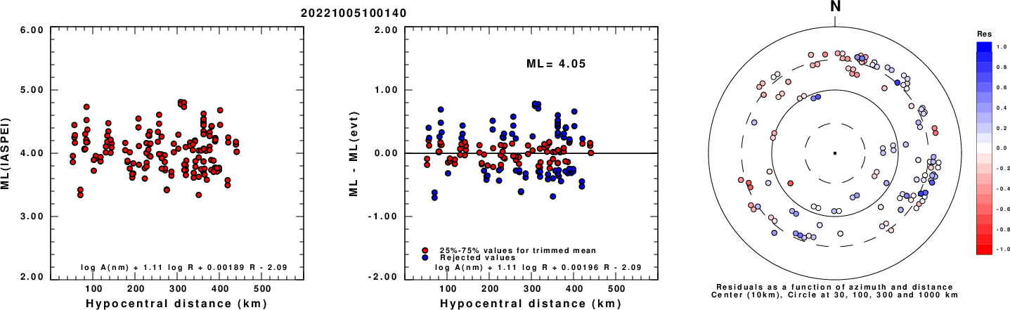
Left: ML computed using the IASPEI formula for Horizontal components. Center: ML residuals computed using a modified IASPEI formula that accounts for path specific attenuation; the values used for the trimmed mean are indicated. The ML relation used for each figure is given at the bottom of each plot.
Right: Residuals from new relation as a function of distance and azimuth.
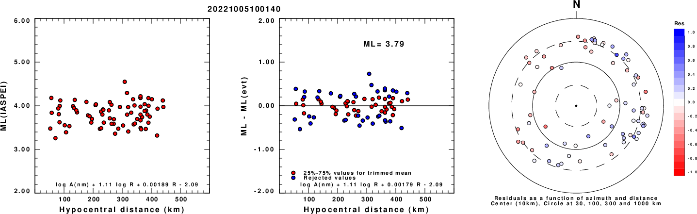
Left: ML computed using the IASPEI formula for Vertical components (research). Center: ML residuals computed using a modified IASPEI formula that accounts for path specific attenuation; the values used for the trimmed mean are indicated. The ML relation used for each figure is given at the bottom of each plot.
Right: Residuals from new relation as a function of distance and azimuth.
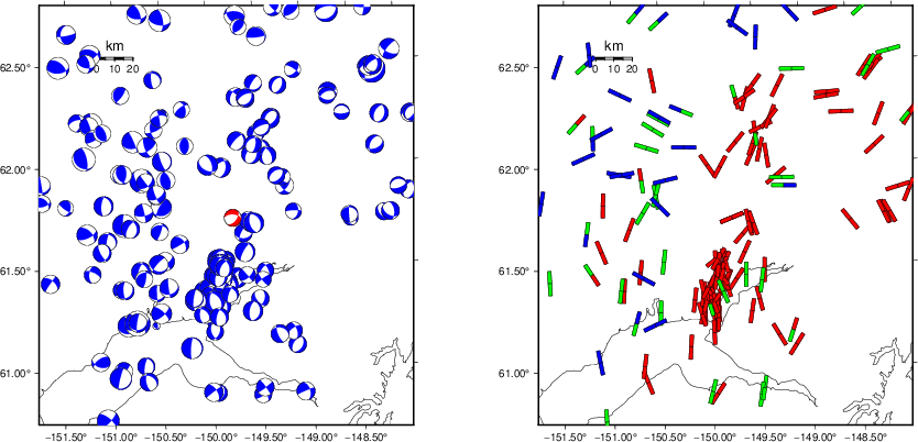
Context
The left panel of the next figure presents the focal mechanism for this earthquake (red) in the context of other nearby events (blue) in the SLU Moment Tensor Catalog. The right panel shows the inferred direction of maximum compressive stress and the type of faulting (green is strike-slip, red is normal, blue is thrust; oblique is shown by a combination of colors). Thus context plot is useful for assessing the appropriateness of the moment tensor of this event.
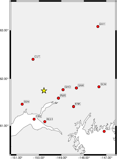
Waveform Inversion using wvfgrd96
The focal mechanism was determined using broadband seismic waveforms. The location of the event (star) and the
stations used for (red) the waveform inversion are shown in the next figure.
|
|
Location of broadband stations used for waveform inversion
|
The program wvfgrd96 was used with good traces observed at short distance to determine the focal mechanism, depth and seismic moment. This technique requires a high quality signal and well determined velocity model for the Green's functions. To the extent that these are the quality data, this type of mechanism should be preferred over the radiation pattern technique which requires the separate step of defining the pressure and tension quadrants and the correct strike.
The observed and predicted traces are filtered using the following gsac commands:
cut o DIST/3.3 -40 o DIST/3.3 +50
rtr
taper w 0.1
hp c 0.03 n 3
lp c 0.08 n 3
The results of this grid search are as follow:
           DEPTH  STK   DIP  RAKE   MW    FIT
WVFGRD96    1.0   160    45    90   3.07 0.1743
WVFGRD96    2.0   340    45    90   3.23 0.2529
WVFGRD96    3.0   310    45    40   3.23 0.2674
WVFGRD96    4.0   300    50    15   3.23 0.2947
WVFGRD96    5.0   300    50    15   3.26 0.3182
WVFGRD96    6.0   300    55    15   3.28 0.3388
WVFGRD96    7.0   295    60     0   3.30 0.3568
WVFGRD96    8.0   300    55    10   3.36 0.3725
WVFGRD96    9.0   295    55     0   3.37 0.3828
WVFGRD96   10.0   295    60     0   3.39 0.3922
WVFGRD96   11.0   295    60     0   3.41 0.3995
WVFGRD96   12.0   295    60     0   3.42 0.4048
WVFGRD96   13.0   295    60     0   3.44 0.4084
WVFGRD96   14.0   295    60     0   3.45 0.4108
WVFGRD96   15.0   295    60     5   3.46 0.4127
WVFGRD96   16.0   295    60     5   3.48 0.4149
WVFGRD96   17.0   295    60     5   3.49 0.4165
WVFGRD96   18.0   295    60     5   3.50 0.4182
WVFGRD96   19.0   295    60     5   3.51 0.4211
WVFGRD96   20.0   295    60     5   3.52 0.4248
WVFGRD96   21.0   295    60     5   3.53 0.4286
WVFGRD96   22.0   295    60     0   3.54 0.4328
WVFGRD96   23.0   295    65    -5   3.55 0.4375
WVFGRD96   24.0   295    65    -5   3.56 0.4413
WVFGRD96   25.0   295    65   -10   3.57 0.4462
WVFGRD96   26.0   290    60   -15   3.58 0.4505
WVFGRD96   27.0   290    60   -15   3.59 0.4557
WVFGRD96   28.0   290    60   -15   3.60 0.4598
WVFGRD96   29.0   290    60   -20   3.61 0.4641
WVFGRD96   30.0   290    60   -20   3.62 0.4679
WVFGRD96   31.0   290    60   -20   3.63 0.4711
WVFGRD96   32.0   290    60   -20   3.63 0.4726
WVFGRD96   33.0   285    60   -30   3.64 0.4747
WVFGRD96   34.0   285    60   -30   3.65 0.4760
WVFGRD96   35.0   285    60   -30   3.66 0.4780
WVFGRD96   36.0   285    60   -30   3.66 0.4781
WVFGRD96   37.0   285    60   -30   3.67 0.4771
WVFGRD96   38.0   285    60   -30   3.68 0.4757
WVFGRD96   39.0   285    65   -35   3.69 0.4734
WVFGRD96   40.0   280    50   -35   3.77 0.4828
WVFGRD96   41.0   280    55   -40   3.77 0.4820
WVFGRD96   42.0   280    55   -40   3.78 0.4818
WVFGRD96   43.0   280    55   -45   3.80 0.4820
WVFGRD96   44.0   275    55   -50   3.80 0.4841
WVFGRD96   45.0   275    55   -50   3.81 0.4848
WVFGRD96   46.0   275    55   -50   3.82 0.4857
WVFGRD96   47.0   275    55   -50   3.82 0.4862
WVFGRD96   48.0   275    55   -50   3.83 0.4863
WVFGRD96   49.0   275    55   -50   3.83 0.4863
WVFGRD96   50.0   275    55   -50   3.83 0.4851
WVFGRD96   51.0   275    55   -50   3.84 0.4862
WVFGRD96   52.0   275    55   -50   3.84 0.4861
WVFGRD96   53.0   275    55   -50   3.85 0.4846
WVFGRD96   54.0   275    55   -50   3.85 0.4846
WVFGRD96   55.0   270    55   -60   3.86 0.4837
WVFGRD96   56.0   270    55   -60   3.86 0.4836
WVFGRD96   57.0   270    55   -60   3.86 0.4829
WVFGRD96   58.0   270    55   -60   3.87 0.4820
WVFGRD96   59.0   270    55   -60   3.87 0.4822
WVFGRD96   60.0   270    55   -60   3.87 0.4806
WVFGRD96   61.0   270    55   -60   3.87 0.4800
WVFGRD96   62.0   275    60   -55   3.86 0.4791
WVFGRD96   63.0   275    60   -55   3.87 0.4776
WVFGRD96   64.0   275    60   -55   3.87 0.4772
WVFGRD96   65.0   275    60   -55   3.87 0.4757
WVFGRD96   66.0   275    60   -55   3.87 0.4751
WVFGRD96   67.0   270    60   -65   3.88 0.4736
WVFGRD96   68.0   270    60   -65   3.88 0.4735
WVFGRD96   69.0   270    60   -65   3.88 0.4728
WVFGRD96   70.0   270    60   -65   3.88 0.4709
WVFGRD96   71.0   270    60   -65   3.88 0.4706
WVFGRD96   72.0   270    60   -65   3.89 0.4694
WVFGRD96   73.0   265    60   -70   3.88 0.4681
WVFGRD96   74.0   265    60   -70   3.89 0.4669
WVFGRD96   75.0   265    60   -70   3.89 0.4660
WVFGRD96   76.0   265    60   -70   3.89 0.4651
WVFGRD96   77.0   265    60   -70   3.89 0.4632
WVFGRD96   78.0   265    60   -70   3.89 0.4626
WVFGRD96   79.0   265    60   -70   3.89 0.4611
WVFGRD96   80.0   265    60   -70   3.90 0.4597
WVFGRD96   81.0   265    60   -70   3.90 0.4580
WVFGRD96   82.0   265    60   -75   3.90 0.4566
WVFGRD96   83.0   260    60   -80   3.90 0.4561
WVFGRD96   84.0   260    60   -80   3.91 0.4537
WVFGRD96   85.0   260    60   -80   3.91 0.4528
WVFGRD96   86.0   260    60   -80   3.91 0.4512
WVFGRD96   87.0   260    60   -80   3.91 0.4502
WVFGRD96   88.0   260    60   -80   3.91 0.4484
WVFGRD96   89.0   260    60   -80   3.91 0.4461
WVFGRD96   90.0   260    60   -80   3.91 0.4452
WVFGRD96   91.0   260    60   -80   3.92 0.4434
WVFGRD96   92.0   260    60   -80   3.92 0.4416
WVFGRD96   93.0   260    60   -80   3.92 0.4397
WVFGRD96   94.0   260    60   -80   3.92 0.4377
WVFGRD96   95.0   260    60   -80   3.92 0.4366
WVFGRD96   96.0   260    60   -80   3.92 0.4341
WVFGRD96   97.0   260    60   -80   3.92 0.4322
WVFGRD96   98.0   260    60   -80   3.92 0.4306
WVFGRD96   99.0   260    60   -80   3.93 0.4286
The best solution is
WVFGRD96 49.0 275 55 -50 3.83 0.4863
The mechanism corresponding to the best fit is
|
|
Figure 1. Waveform inversion focal mechanism
|
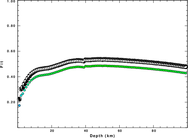
The best fit as a function of depth is given in the following figure:
|
|
Figure 2. Depth sensitivity for waveform mechanism
|
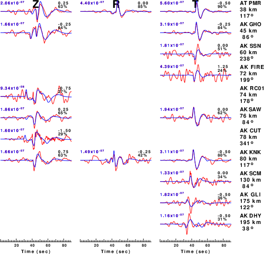
The comparison of the observed and predicted waveforms is given in the next figure. The red traces are the observed and the blue are the predicted.
Each observed-predicted component is plotted to the same scale and peak amplitudes are indicated by the numbers to the left of each trace. A pair of numbers is given in black at the right of each predicted traces. The upper number it the time shift required for maximum correlation between the observed and predicted traces. This time shift is required because the synthetics are not computed at exactly the same distance as the observed, the velocity model used in the predictions may not be perfect and the epicentral parameters may be be off.
A positive time shift indicates that the prediction is too fast and should be delayed to match the observed trace (shift to the right in this figure). A negative value indicates that the prediction is too slow. The lower number gives the percentage of variance reduction to characterize the individual goodness of fit (100% indicates a perfect fit).
The bandpass filter used in the processing and for the display was
cut o DIST/3.3 -40 o DIST/3.3 +50
rtr
taper w 0.1
hp c 0.03 n 3
lp c 0.08 n 3
|
|
Figure 3. Waveform comparison for selected depth. Red: observed; Blue - predicted. The time shift with respect to the model prediction is indicated. The percent of fit is also indicated. The time scale is relative to the first trace sample.
|
|
|
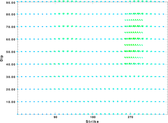
Focal mechanism sensitivity at the preferred depth. The red color indicates a very good fit to the waveforms.
Each solution is plotted as a vector at a given value of strike and dip with the angle of the vector representing the rake angle, measured, with respect to the upward vertical (N) in the figure.
|
A check on the assumed source location is possible by looking at the time shifts between the observed and predicted traces. The time shifts for waveform matching arise for several reasons:
- The origin time and epicentral distance are incorrect
- The velocity model used for the inversion is incorrect
- The velocity model used to define the P-arrival time is not the
same as the velocity model used for the waveform inversion
(assuming that the initial trace alignment is based on the
P arrival time)
Assuming only a mislocation, the time shifts are fit to a functional form:
Time_shift = A + B cos Azimuth + C Sin Azimuth
The time shifts for this inversion lead to the next figure:
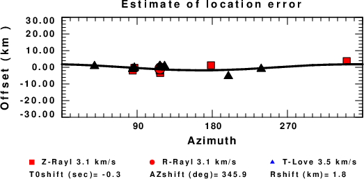
The derived shift in origin time and epicentral coordinates are given at the bottom of the figure.
Velocity Model
The WUS.model used for the waveform synthetic seismograms and for the surface wave eigenfunctions and dispersion is as follows
(The format is in the model96 format of Computer Programs in Seismology).
MODEL.01
Model after     8 iterations
ISOTROPIC
KGS
FLAT EARTH
1-D
CONSTANT VELOCITY
LINE08
LINE09
LINE10
LINE11
      H(KM)   VP(KM/S)   VS(KM/S) RHO(GM/CC)         QP         QS       ETAP       ETAS      FREFP      FREFS
     1.9000     3.4065     2.0089     2.2150  0.302E-02  0.679E-02   0.00       0.00       1.00       1.00
     6.1000     5.5445     3.2953     2.6089  0.349E-02  0.784E-02   0.00       0.00       1.00       1.00
    13.0000     6.2708     3.7396     2.7812  0.212E-02  0.476E-02   0.00       0.00       1.00       1.00
    19.0000     6.4075     3.7680     2.8223  0.111E-02  0.249E-02   0.00       0.00       1.00       1.00
     0.0000     7.9000     4.6200     3.2760  0.164E-10  0.370E-10   0.00       0.00       1.00       1.00
Last Changed Thu Apr 25 01:30:27 AM CDT 2024