Location

Location ANSS

The ANSS event ID is ak02196xqxn5 and the event page is at https://earthquake.usgs.gov/earthquakes/eventpage/ak02196xqxn5/executive.

2021/07/19 10:52:20 60.223 -151.823 69.9 4.3 Alaska

Focal Mechanism

USGS/SLU Moment Tensor Solution ENS 2021/07/19 10:52:20:0 60.22 -151.82 69.9 4.3 Alaska Stations used: AK.BRLK AK.CAST AK.CNP AK.CUT AK.FID AK.FIRE AK.GHO AK.HOM AK.K20K AK.M20K AK.N18K AK.N19K AK.O18K AK.O19K AK.PPLA AK.PWL AK.Q19K AK.RC01 AK.SAW AK.SKN AK.SLK AK.SWD AK.TRF AV.ILS AV.RED AV.SPCP AV.STLK Filtering commands used: cut o DIST/3.3 -40 o DIST/3.3 +50 rtr taper w 0.1 hp c 0.03 n 3 lp c 0.10 n 3 Best Fitting Double Couple Mo = 2.79e+22 dyne-cm Mw = 4.23 Z = 70 km Plane Strike Dip Rake NP1 10 75 -25 NP2 107 66 -164 Principal Axes: Axis Value Plunge Azimuth T 2.79e+22 6 60 N 0.00e+00 61 161 P -2.79e+22 28 327 Moment Tensor: (dyne-cm) Component Value Mxx -8.16e+21 Mxy 2.19e+22 Mxz -8.21e+21 Myy 1.41e+22 Myz 8.91e+21 Mzz -5.89e+21 -----------### ---------------####### -------------------######### ----- ------------########## ------- P ------------########## -------- ------------########## T ------------------------########## # -------------------------############### #------------------------############### ####---------------------################# ######-------------------################# ########-----------------################# ############------------################## ###############--------################# ####################---################- #####################----------------- ###################----------------- ##################---------------- ###############--------------- #############--------------- #########------------- ####---------- Global CMT Convention Moment Tensor: R T P -5.89e+21 -8.21e+21 -8.91e+21 -8.21e+21 -8.16e+21 -2.19e+22 -8.91e+21 -2.19e+22 1.41e+22 Details of the solution is found at http://www.eas.slu.edu/eqc/eqc_mt/MECH.NA/20210719105220/index.html

Preferred Solution

The preferred solution from an analysis of the surface-wave spectral amplitude radiation pattern, waveform inversion or first motion observations is

      STK = 10
      DIP = 75
     RAKE = -25
       MW = 4.23
       HS = 70.0

The NDK file is 20210719105220.ndk The waveform inversion is preferred.

Magnitudes

Given the availability of digital waveforms for determination of the moment tensor, this section documents the added processing leading to mLg, if appropriate to the region, and M_L by application of the respective IASPEI formulae. As a research study, the linear distance term of the IASPEI formula for M_L is adjusted to remove a linear distance trend in residuals to give a regionally defined M_L. The defined M_L uses horizontal component recordings, but the same procedure is applied to the vertical components since there may be some interest in vertical component ground motions. Residual plots versus distance may indicate interesting features of ground motion scaling in some distance ranges. A residual plot of the regionalized magnitude is given as a function of distance and azimuth, since data sets may transcend different wave propagation provinces.

ML Magnitude

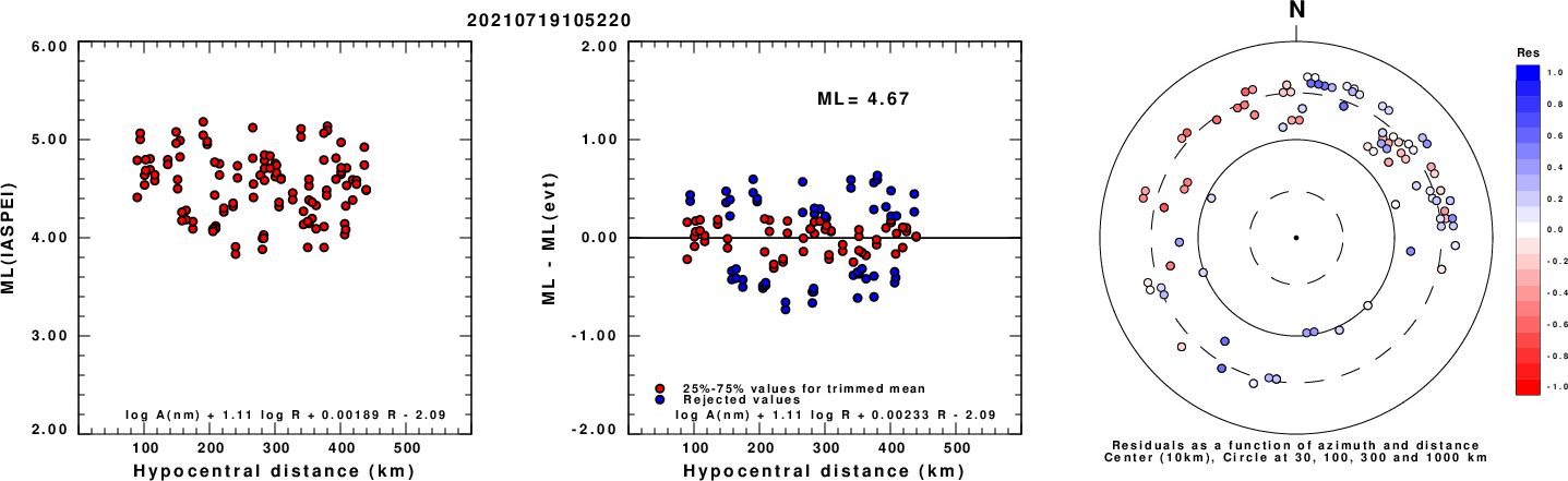
Left: ML computed using the IASPEI formula for Horizontal components. Center: ML residuals computed using a modified IASPEI formula that accounts for path specific attenuation; the values used for the trimmed mean are indicated. The ML relation used for each figure is given at the bottom of each plot. Right: Residuals from new relation as a function of distance and azimuth.

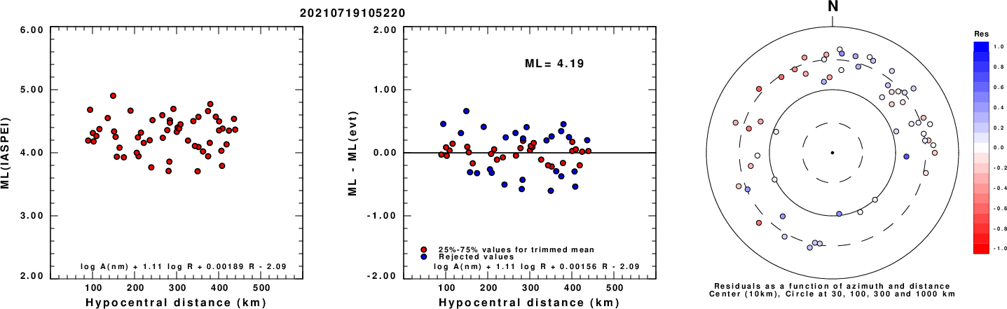
Left: ML computed using the IASPEI formula for Vertical components (research). Center: ML residuals computed using a modified IASPEI formula that accounts for path specific attenuation; the values used for the trimmed mean are indicated. The ML relation used for each figure is given at the bottom of each plot. Right: Residuals from new relation as a function of distance and azimuth.

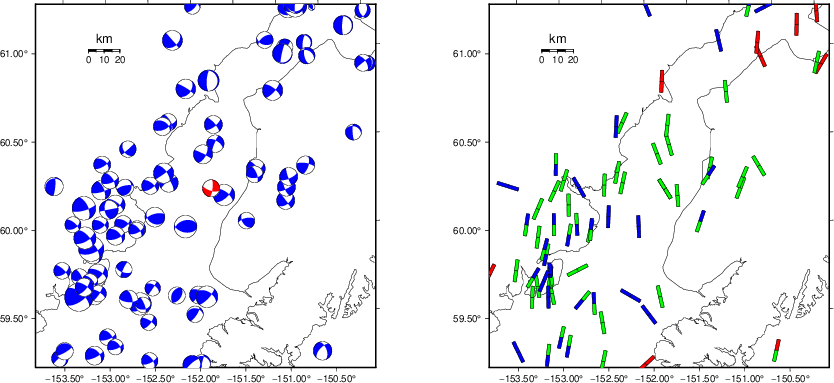
Context

The left panel of the next figure presents the focal mechanism for this earthquake (red) in the context of other nearby events (blue) in the SLU Moment Tensor Catalog. The right panel shows the inferred direction of maximum compressive stress and the type of faulting (green is strike-slip, red is normal, blue is thrust; oblique is shown by a combination of colors). Thus context plot is useful for assessing the appropriateness of the moment tensor of this event.

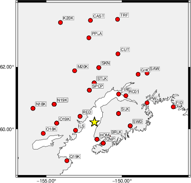
Waveform Inversion using wvfgrd96

The focal mechanism was determined using broadband seismic waveforms. The location of the event (star) and the stations used for (red) the waveform inversion are shown in the next figure.

Location of broadband stations used for waveform inversion

The program wvfgrd96 was used with good traces observed at short distance to determine the focal mechanism, depth and seismic moment. This technique requires a high quality signal and well determined velocity model for the Green's functions. To the extent that these are the quality data, this type of mechanism should be preferred over the radiation pattern technique which requires the separate step of defining the pressure and tension quadrants and the correct strike.

The observed and predicted traces are filtered using the following gsac commands:

cut o DIST/3.3 -40 o DIST/3.3 +50
rtr
taper w 0.1
hp c 0.03 n 3 
lp c 0.10 n 3

The results of this grid search are as follow:

           DEPTH  STK   DIP  RAKE   MW    FIT
WVFGRD96    2.0   105    60    25   3.36 0.2296
WVFGRD96    4.0   275    75   -10   3.42 0.2641
WVFGRD96    6.0   100    70    10   3.49 0.2796
WVFGRD96    8.0    95    70   -10   3.57 0.2908
WVFGRD96   10.0    95    70   -10   3.61 0.2889
WVFGRD96   12.0    95    70    -5   3.64 0.2793
WVFGRD96   14.0     5    80   -10   3.68 0.2731
WVFGRD96   16.0     5    80   -10   3.71 0.2826
WVFGRD96   18.0     5    80   -10   3.74 0.2948
WVFGRD96   20.0     5    80   -15   3.77 0.3127
WVFGRD96   22.0     5    80   -15   3.80 0.3323
WVFGRD96   24.0     5    80   -10   3.83 0.3531
WVFGRD96   26.0     5    80   -15   3.85 0.3743
WVFGRD96   28.0     5    80   -15   3.87 0.3955
WVFGRD96   30.0     5    80   -10   3.89 0.4156
WVFGRD96   32.0     5    80   -10   3.90 0.4348
WVFGRD96   34.0     5    80   -10   3.92 0.4471
WVFGRD96   36.0     5    80   -15   3.94 0.4613
WVFGRD96   38.0     5    80   -15   3.97 0.4724
WVFGRD96   40.0     5    75   -20   4.04 0.4897
WVFGRD96   42.0     5    75   -20   4.06 0.4938
WVFGRD96   44.0     5    75   -20   4.08 0.5020
WVFGRD96   46.0     5    75   -20   4.10 0.5084
WVFGRD96   48.0     5    75   -20   4.12 0.5175
WVFGRD96   50.0     5    75   -20   4.13 0.5257
WVFGRD96   52.0     5    75   -20   4.14 0.5315
WVFGRD96   54.0    10    80   -20   4.16 0.5388
WVFGRD96   56.0    10    75   -20   4.18 0.5478
WVFGRD96   58.0    10    75   -20   4.19 0.5563
WVFGRD96   60.0    10    75   -20   4.20 0.5626
WVFGRD96   62.0    10    75   -20   4.20 0.5683
WVFGRD96   64.0    10    75   -20   4.21 0.5737
WVFGRD96   66.0    10    75   -25   4.22 0.5774
WVFGRD96   68.0    10    75   -25   4.23 0.5801
WVFGRD96   70.0    10    75   -25   4.23 0.5818
WVFGRD96   72.0    10    75   -25   4.24 0.5811
WVFGRD96   74.0    10    75   -25   4.24 0.5801
WVFGRD96   76.0    10    75   -25   4.25 0.5785
WVFGRD96   78.0    10    75   -25   4.25 0.5765
WVFGRD96   80.0    10    75   -25   4.25 0.5729
WVFGRD96   82.0    10    75   -25   4.26 0.5699
WVFGRD96   84.0    10    75   -25   4.26 0.5638
WVFGRD96   86.0    10    75   -25   4.26 0.5591
WVFGRD96   88.0    10    75   -25   4.27 0.5545
WVFGRD96   90.0    10    75   -25   4.27 0.5482
WVFGRD96   92.0    10    75   -25   4.27 0.5427
WVFGRD96   94.0    10    75   -25   4.27 0.5374
WVFGRD96   96.0    10    75   -25   4.27 0.5308
WVFGRD96   98.0    10    75   -25   4.28 0.5267
WVFGRD96  100.0    10    75   -25   4.28 0.5218
WVFGRD96  102.0    10    75   -25   4.28 0.5163
WVFGRD96  104.0    10    75   -25   4.28 0.5123
WVFGRD96  106.0    10    75   -25   4.29 0.5067
WVFGRD96  108.0    10    75   -25   4.29 0.5031
WVFGRD96  110.0    10    75   -25   4.29 0.4990
WVFGRD96  112.0    10    75   -25   4.29 0.4944
WVFGRD96  114.0    10    75   -25   4.30 0.4902
WVFGRD96  116.0    10    75   -25   4.30 0.4858
WVFGRD96  118.0    10    75   -25   4.30 0.4826
WVFGRD96  120.0    10    75   -25   4.30 0.4767
WVFGRD96  122.0    10    75   -25   4.30 0.4728
WVFGRD96  124.0    10    75   -25   4.31 0.4648
WVFGRD96  126.0    10    75   -25   4.31 0.4561
WVFGRD96  128.0    -5    70   -35   4.29 0.4409
WVFGRD96  130.0    -5    70   -35   4.29 0.4300
WVFGRD96  132.0    -5    70   -35   4.29 0.4174
WVFGRD96  134.0   355    70   -35   4.29 0.4025
WVFGRD96  136.0   350    65   -35   4.28 0.3633
WVFGRD96  138.0    -5    60   -30   4.27 0.3065
WVFGRD96  140.0    10    85     0   4.23 0.2572
WVFGRD96  142.0    15    85    55   4.22 0.2522
WVFGRD96  144.0    15    85    55   4.22 0.2491
WVFGRD96  146.0    15    80    65   4.22 0.2472
WVFGRD96  148.0    15    80    65   4.23 0.2461

The best solution is

WVFGRD96   70.0    10    75   -25   4.23 0.5818

The mechanism corresponding to the best fit is

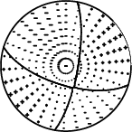
Figure 1. Waveform inversion focal mechanism

The best fit as a function of depth is given in the following figure:

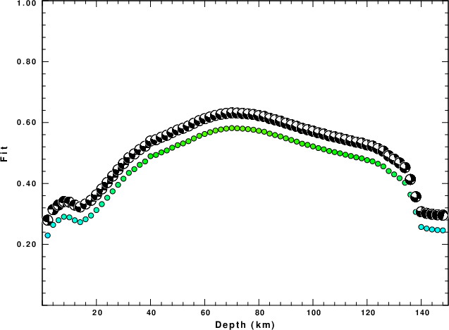
Figure 2. Depth sensitivity for waveform mechanism

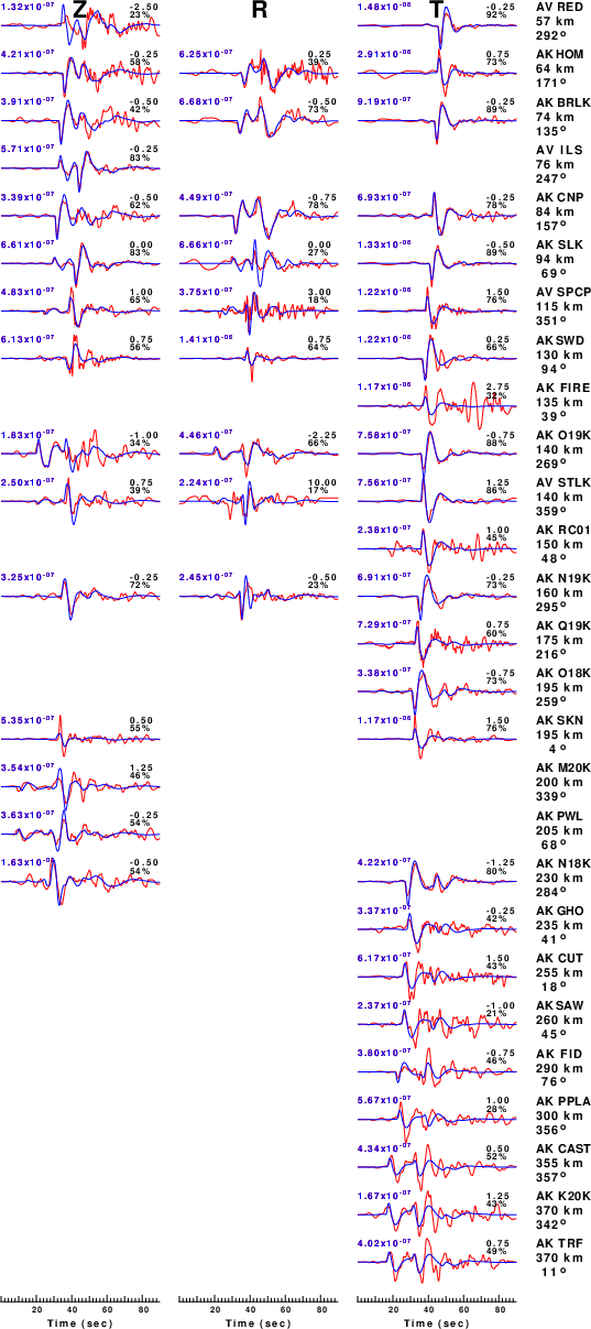
The comparison of the observed and predicted waveforms is given in the next figure. The red traces are the observed and the blue are the predicted. Each observed-predicted component is plotted to the same scale and peak amplitudes are indicated by the numbers to the left of each trace. A pair of numbers is given in black at the right of each predicted traces. The upper number it the time shift required for maximum correlation between the observed and predicted traces. This time shift is required because the synthetics are not computed at exactly the same distance as the observed, the velocity model used in the predictions may not be perfect and the epicentral parameters may be be off. A positive time shift indicates that the prediction is too fast and should be delayed to match the observed trace (shift to the right in this figure). A negative value indicates that the prediction is too slow. The lower number gives the percentage of variance reduction to characterize the individual goodness of fit (100% indicates a perfect fit).

The bandpass filter used in the processing and for the display was

cut o DIST/3.3 -40 o DIST/3.3 +50
rtr
taper w 0.1
hp c 0.03 n 3 
lp c 0.10 n 3

Figure 3. Waveform comparison for selected depth. Red: observed; Blue - predicted. The time shift with respect to the model prediction is indicated. The percent of fit is also indicated. The time scale is relative to the first trace sample.

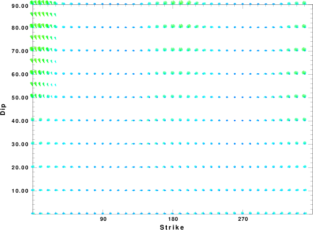
Focal mechanism sensitivity at the preferred depth. The red color indicates a very good fit to the waveforms. Each solution is plotted as a vector at a given value of strike and dip with the angle of the vector representing the rake angle, measured, with respect to the upward vertical (N) in the figure.

A check on the assumed source location is possible by looking at the time shifts between the observed and predicted traces. The time shifts for waveform matching arise for several reasons:

The origin time and epicentral distance are incorrect
The velocity model used for the inversion is incorrect
The velocity model used to define the P-arrival time is not the same as the velocity model used for the waveform inversion (assuming that the initial trace alignment is based on the P arrival time)

Assuming only a mislocation, the time shifts are fit to a functional form:

 Time_shift = A + B cos Azimuth + C Sin Azimuth

The time shifts for this inversion lead to the next figure:

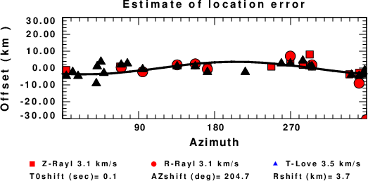
The derived shift in origin time and epicentral coordinates are given at the bottom of the figure.

Velocity Model

The WUS.model used for the waveform synthetic seismograms and for the surface wave eigenfunctions and dispersion is as follows (The format is in the model96 format of Computer Programs in Seismology).

MODEL.01
Model after     8 iterations
ISOTROPIC
KGS
FLAT EARTH
1-D
CONSTANT VELOCITY
LINE08
LINE09
LINE10
LINE11
      H(KM)   VP(KM/S)   VS(KM/S) RHO(GM/CC)         QP         QS       ETAP       ETAS      FREFP      FREFS
     1.9000     3.4065     2.0089     2.2150  0.302E-02  0.679E-02   0.00       0.00       1.00       1.00    
     6.1000     5.5445     3.2953     2.6089  0.349E-02  0.784E-02   0.00       0.00       1.00       1.00    
    13.0000     6.2708     3.7396     2.7812  0.212E-02  0.476E-02   0.00       0.00       1.00       1.00    
    19.0000     6.4075     3.7680     2.8223  0.111E-02  0.249E-02   0.00       0.00       1.00       1.00    
     0.0000     7.9000     4.6200     3.2760  0.164E-10  0.370E-10   0.00       0.00       1.00       1.00

Last Changed Thu Apr 25 12:25:51 AM CDT 2024