Location
Location ANSS
The ANSS event ID is uw61730837 and the event page is at
https://earthquake.usgs.gov/earthquakes/eventpage/uw61730837/executive.
2021/06/06 03:51:37 45.342 -121.694 4.3 3.94 Oregon
Focal Mechanism
 USGS/SLU Moment Tensor Solution
 ENS  2021/06/06 03:51:37:0  45.34 -121.69   4.3 3.9 Oregon

 Stations used:
   CC.JRO IU.COR UO.ALSE UO.BEER UO.BUCK UO.CAVE UO.DBO
   UO.DFAZ UO.DRAN UO.FHAC UO.JESE UO.LAIR UO.MARQ UO.MINN
   UO.NATH UO.PF27 UO.PINE UO.RAIN UO.ROGE UO.UCHR UO.WLOO
   US.BMO US.HAWA US.NLWA US.WVOR UW.BBO UW.BLOW UW.CCRK
   UW.DDRF UW.DEAL UW.EPH2 UW.FISH UW.GNW UW.HILL UW.IRON
   UW.IZEE UW.JEDS UW.KENT UW.LBRT UW.LCCR UW.LEBA UW.LNO
   UW.LON UW.LRIV UW.LTY UW.MOX UW.OMAK UW.PAN4H UW.PHIN
   UW.RADR UW.STOR UW.TOLE UW.TUCA UW.UMAT UW.WA2 UW.WOLL
   UW.YPT

 Filtering commands used:
   cut o DIST/3.3 -40 o DIST/3.3 +50
   rtr
   taper w 0.1
   hp c 0.03 n 3
   lp c 0.10 n 3
   br c 0.12 0.25 n 4 p 2

 Best Fitting Double Couple
  Mo = 1.10e+22 dyne-cm
  Mw = 3.96
  Z  = 11 km
  Plane   Strike  Dip  Rake
   NP1      323    71   159
   NP2       60    70    20
  Principal Axes:
   Axis    Value   Plunge  Azimuth
    T   1.10e+22     28     281
    N   0.00e+00     62     103
    P  -1.10e+22      1      12

 Moment Tensor: (dyne-cm)
    Component   Value
       Mxx    -1.02e+22
       Mxy    -3.80e+21
       Mxz     7.26e+20
       Myy     7.78e+21
       Myz    -4.49e+21
       Mzz     2.41e+21


                     ---------- P -
                 --------------   -----
              ####------------------------
             ########----------------------
           ############----------------------
          ###############---------------------
         ##################------------------##
        #####################---------------####
        ####   ###############------------######
       ##### T #################--------#########
       #####   ##################-----###########
       ###########################--#############
       ##########################---#############
        ######################-------###########
        ###################-----------##########
         #############----------------#########
          #####------------------------#######
           -----------------------------#####
             ---------------------------###
              --------------------------##
                 ----------------------
                     --------------


 Global CMT Convention Moment Tensor:
      R          T          P
  2.41e+21   7.26e+20   4.49e+21
  7.26e+20  -1.02e+22   3.80e+21
  4.49e+21   3.80e+21   7.78e+21


Details of the solution is found at

http://www.eas.slu.edu/eqc/eqc_mt/MECH.NA/20210606035137/index.html
|
Preferred Solution
The preferred solution from an analysis of the surface-wave spectral amplitude radiation pattern, waveform inversion or first motion observations is
      STK = 60
      DIP = 70
     RAKE = 20
       MW = 3.96
       HS = 11.0
The NDK file is 20210606035137.ndk
The waveform inversion is preferred.
Magnitudes
Given the availability of digital waveforms for determination of the moment tensor, this section documents the added processing leading to mLg, if appropriate to the region, and ML by application of the respective IASPEI formulae. As a research study, the linear distance term of the IASPEI formula
for ML is adjusted to remove a linear distance trend in residuals to give a regionally defined ML. The defined ML uses horizontal component recordings, but the same procedure is applied to the vertical components since there may be some interest in vertical component ground motions. Residual plots versus distance may indicate interesting features of ground motion scaling in some distance ranges. A residual plot of the regionalized magnitude is given as a function of distance and azimuth, since data sets may transcend different wave propagation provinces.
ML Magnitude
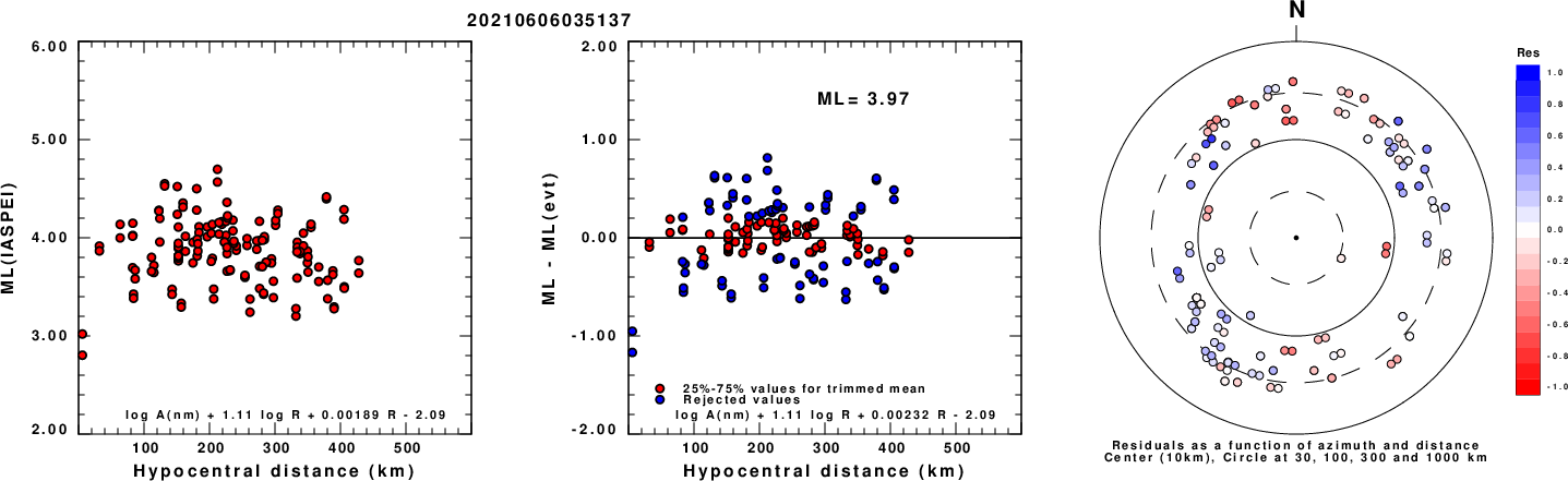
Left: ML computed using the IASPEI formula for Horizontal components. Center: ML residuals computed using a modified IASPEI formula that accounts for path specific attenuation; the values used for the trimmed mean are indicated. The ML relation used for each figure is given at the bottom of each plot.
Right: Residuals from new relation as a function of distance and azimuth.
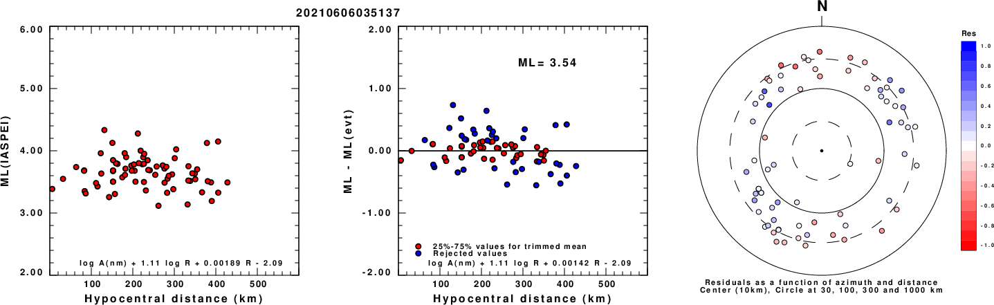
Left: ML computed using the IASPEI formula for Vertical components (research). Center: ML residuals computed using a modified IASPEI formula that accounts for path specific attenuation; the values used for the trimmed mean are indicated. The ML relation used for each figure is given at the bottom of each plot.
Right: Residuals from new relation as a function of distance and azimuth.
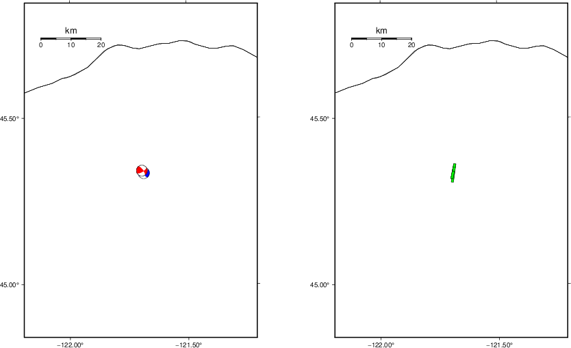
Context
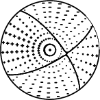
The left panel of the next figure presents the focal mechanism for this earthquake (red) in the context of other nearby events (blue) in the SLU Moment Tensor Catalog. The right panel shows the inferred direction of maximum compressive stress and the type of faulting (green is strike-slip, red is normal, blue is thrust; oblique is shown by a combination of colors). Thus context plot is useful for assessing the appropriateness of the moment tensor of this event.
Waveform Inversion using wvfgrd96
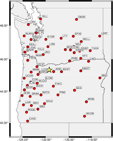
The focal mechanism was determined using broadband seismic waveforms. The location of the event (star) and the
stations used for (red) the waveform inversion are shown in the next figure.
|
|
Location of broadband stations used for waveform inversion
|
The program wvfgrd96 was used with good traces observed at short distance to determine the focal mechanism, depth and seismic moment. This technique requires a high quality signal and well determined velocity model for the Green's functions. To the extent that these are the quality data, this type of mechanism should be preferred over the radiation pattern technique which requires the separate step of defining the pressure and tension quadrants and the correct strike.
The observed and predicted traces are filtered using the following gsac commands:
cut o DIST/3.3 -40 o DIST/3.3 +50
rtr
taper w 0.1
hp c 0.03 n 3
lp c 0.10 n 3
br c 0.12 0.25 n 4 p 2
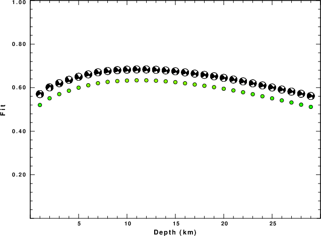
The results of this grid search are as follow:
           DEPTH  STK   DIP  RAKE   MW    FIT
WVFGRD96    1.0   235    85   -30   3.85 0.5204
WVFGRD96    2.0   230    75   -35   3.89 0.5513
WVFGRD96    3.0    55    65    -5   3.88 0.5704
WVFGRD96    4.0    55    60    -5   3.90 0.5860
WVFGRD96    5.0    55    60    -5   3.91 0.5999
WVFGRD96    6.0    60    65    15   3.92 0.6110
WVFGRD96    7.0    60    65    15   3.93 0.6204
WVFGRD96    8.0    60    65    15   3.93 0.6265
WVFGRD96    9.0    60    70    20   3.94 0.6302
WVFGRD96   10.0    60    65    15   3.95 0.6325
WVFGRD96   11.0    60    70    20   3.96 0.6337
WVFGRD96   12.0    60    70    15   3.97 0.6336
WVFGRD96   13.0    60    70    15   3.97 0.6321
WVFGRD96   14.0    60    70    15   3.98 0.6290
WVFGRD96   15.0    60    70    15   3.99 0.6252
WVFGRD96   16.0    60    70    15   4.00 0.6201
WVFGRD96   17.0    55    75    10   4.01 0.6145
WVFGRD96   18.0    55    75    15   4.02 0.6087
WVFGRD96   19.0    55    75    15   4.03 0.6022
WVFGRD96   20.0    60    70    20   4.04 0.5950
WVFGRD96   21.0    60    70    20   4.05 0.5873
WVFGRD96   22.0    60    70    20   4.05 0.5789
WVFGRD96   23.0    60    70    20   4.06 0.5698
WVFGRD96   24.0    60    70    20   4.07 0.5604
WVFGRD96   25.0    60    70    25   4.08 0.5509
WVFGRD96   26.0    60    70    25   4.09 0.5414
WVFGRD96   27.0    60    70    25   4.09 0.5319
WVFGRD96   28.0    60    70    25   4.10 0.5220
WVFGRD96   29.0    60    70    25   4.11 0.5117
The best solution is
WVFGRD96 11.0 60 70 20 3.96 0.6337
The mechanism corresponding to the best fit is
|
|
Figure 1. Waveform inversion focal mechanism
|
The best fit as a function of depth is given in the following figure:
|
|
Figure 2. Depth sensitivity for waveform mechanism
|
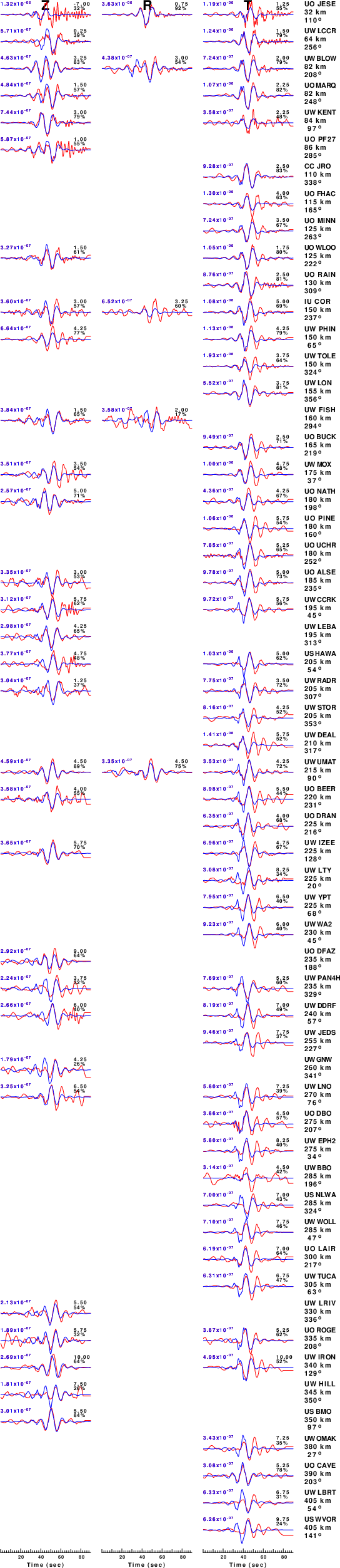
The comparison of the observed and predicted waveforms is given in the next figure. The red traces are the observed and the blue are the predicted.
Each observed-predicted component is plotted to the same scale and peak amplitudes are indicated by the numbers to the left of each trace. A pair of numbers is given in black at the right of each predicted traces. The upper number it the time shift required for maximum correlation between the observed and predicted traces. This time shift is required because the synthetics are not computed at exactly the same distance as the observed, the velocity model used in the predictions may not be perfect and the epicentral parameters may be be off.
A positive time shift indicates that the prediction is too fast and should be delayed to match the observed trace (shift to the right in this figure). A negative value indicates that the prediction is too slow. The lower number gives the percentage of variance reduction to characterize the individual goodness of fit (100% indicates a perfect fit).
The bandpass filter used in the processing and for the display was
cut o DIST/3.3 -40 o DIST/3.3 +50
rtr
taper w 0.1
hp c 0.03 n 3
lp c 0.10 n 3
br c 0.12 0.25 n 4 p 2
|
|
Figure 3. Waveform comparison for selected depth. Red: observed; Blue - predicted. The time shift with respect to the model prediction is indicated. The percent of fit is also indicated. The time scale is relative to the first trace sample.
|
|
|
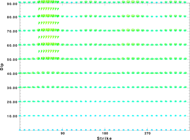
Focal mechanism sensitivity at the preferred depth. The red color indicates a very good fit to the waveforms.
Each solution is plotted as a vector at a given value of strike and dip with the angle of the vector representing the rake angle, measured, with respect to the upward vertical (N) in the figure.
|
A check on the assumed source location is possible by looking at the time shifts between the observed and predicted traces. The time shifts for waveform matching arise for several reasons:
- The origin time and epicentral distance are incorrect
- The velocity model used for the inversion is incorrect
- The velocity model used to define the P-arrival time is not the
same as the velocity model used for the waveform inversion
(assuming that the initial trace alignment is based on the
P arrival time)
Assuming only a mislocation, the time shifts are fit to a functional form:
Time_shift = A + B cos Azimuth + C Sin Azimuth
The time shifts for this inversion lead to the next figure:
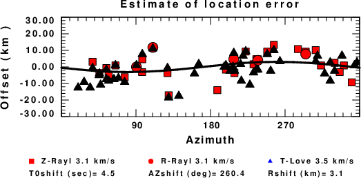
The derived shift in origin time and epicentral coordinates are given at the bottom of the figure.
Velocity Model
The CUS.model used for the waveform synthetic seismograms and for the surface wave eigenfunctions and dispersion is as follows
(The format is in the model96 format of Computer Programs in Seismology).
MODEL.01
CUS Model with Q from simple gamma values
ISOTROPIC
KGS
FLAT EARTH
1-D
CONSTANT VELOCITY
LINE08
LINE09
LINE10
LINE11
  H(KM) VP(KM/S) VS(KM/S) RHO(GM/CC)   QP   QS  ETAP  ETAS  FREFP  FREFS
  1.0000  5.0000  2.8900  2.5000 0.172E-02 0.387E-02 0.00  0.00  1.00  1.00
  9.0000  6.1000  3.5200  2.7300 0.160E-02 0.363E-02 0.00  0.00  1.00  1.00
 10.0000  6.4000  3.7000  2.8200 0.149E-02 0.336E-02 0.00  0.00  1.00  1.00
 20.0000  6.7000  3.8700  2.9020 0.000E-04 0.000E-04 0.00  0.00  1.00  1.00
  0.0000  8.1500  4.7000  3.3640 0.194E-02 0.431E-02 0.00  0.00  1.00  1.00
Last Changed Wed Apr 24 11:16:41 PM CDT 2024